Topic 6.8 Notes – Confidence Intervals for the Difference of Two Proportions

Confidence Interval for the Difference of Two Proportions

When you’re comparing two percentages, the parameter is:

$$p_1 - p_2$$

That means the true difference between two population proportions.

The procedure we use is a two-sample z-interval for $p_1 - p_2$.

You use it when:

• There is one categorical variable (success/failure),
• Measured in two independent groups,
• From two random samples or a randomized experiment.

Your estimate is:

$$\hat{p}_1 - \hat{p}_2$$

If the interval includes 0, a difference of 0 is plausible.
If 0 is not in the interval, there’s evidence of a real difference.

Conditions for Inference

You must check all conditions for both samples. Missing even one piece costs points.

1. Random

• Two independent random samples
  or
  Random assignment in an experiment

You must say how randomness happened (quote the scenario).

2. Independence

• The two groups must be independent of each other.
• If sampling without replacement, check the 10% condition for both groups:

$$n_1 \le 0.1N_1 \quad \text{and} \quad n_2 \le 0.1N_2$$

This ensures observations within each sample are independent.

3. Large Counts (Normal Condition)

Check all four:

$$n_1\hat{p}_1 \ge 10$$

$$n_1(1-\hat{p}_1) \ge 10$$

$$n_2\hat{p}_2 \ge 10$$

$$n_2(1-\hat{p}_2) \ge 10$$

These confirm the sampling distribution of $\hat{p}_1 - \hat{p}_2$ is approximately normal.

Students often forget to check all four inequalities.

How the Interval Is Built

A confidence interval always follows:

$$\text{Point Estimate} \pm \text{Margin of Error}$$

Step-by-step

1. Compute sample proportions
   $$\hat{p}_1 = \frac{x_1}{n_1}, \quad \hat{p}_2 = \frac{x_2}{n_2}$$

2. Point estimate
   $$\hat{p}_1 - \hat{p}_2$$

3. Standard error
   $$SE = \sqrt{\frac{\hat{p}_1(1-\hat{p}_1)}{n_1} + \frac{\hat{p}_2(1-\hat{p}_2)}{n_2}}$$

4. Critical value $z^*$

   • 90% → 1.645
   • 95% → 1.96
   • 99% → 2.576

5. Margin of error
   $$ME = z^* \cdot SE$$

6. Final interval
   $$(\hat{p}_1 - \hat{p}_2) \pm ME$$

On your calculator: 2-PropZInt (enter successes and sample sizes).

Notice this standard error is not pooled. Pooled standard error is for hypothesis tests, not confidence intervals. That mix-up shows up a lot on quizzes.

What the Formula Is Really Doing

Here’s the structure clearly. Think of it as point estimate ± margin of error:

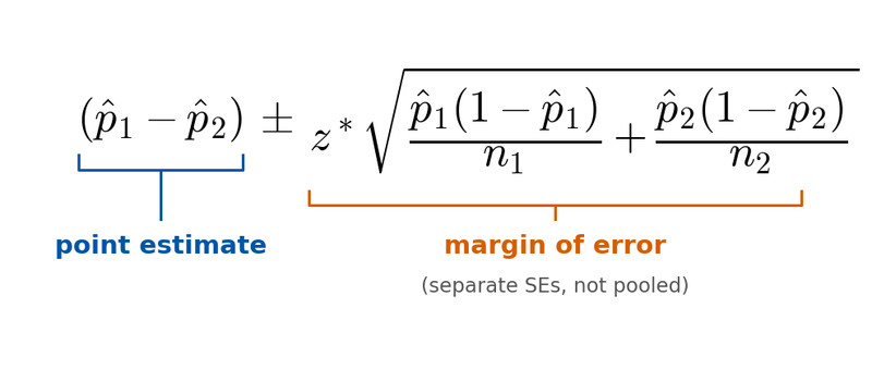
The left side is your sample difference, $\hat{p}_1 - \hat{p}_2$. The right side is how much uncertainty you allow around that difference.

Everything comes from sampling variability of each proportion. The variability from both groups adds together inside the square root.

Also remember: the formula is not printed exactly like this on the AP formula sheet. But it can be built from the provided standard error formulas.

Interpreting in Context

Suppose your interval is:

$$(0.04,\; 0.12)$$

A correct interpretation sounds like:

We are 95% confident that the true difference in the proportion of registered voters who support Candidate A in City 1 compared to City 2 is between 0.04 and 0.12.

Key details:

• State the confidence level
• Mention true population proportions
• Name the groups
• Keep the order consistent with $p_1 - p_2$

If the interval is entirely positive, group 1 likely has the higher proportion.
If entirely negative, group 2 likely does.
If it contains 0, there’s no convincing evidence of a difference.

Never say “there is a 95% probability the true difference is in this interval.” The parameter is fixed.

Using the Interval to Estimate Differences

The endpoints tell you how far apart the groups might realistically be.

If your interval is: $$(-0.03,\; 0.08)$$

That means the difference could range from 3 percentage points lower to 8 percentage points higher for group 1. Always interpret in percentage points, not percent increase.

On free-response questions, direction matters. If you define $p_1 - p_2$, stick with that order the entire time.