Topic 8.1 Notes – Introducing Statistics: Are My Results Unexpected?

When Observed Counts Don’t Match Expected Counts

In categorical data, we deal with counts in categories.

• Observed counts (O) are what you actually saw in your sample.
• Expected counts (E) are what you would predict if some claim or model were true.

For example, suppose a company claims that 30% of customers prefer Product A, 50% prefer B, and 20% prefer C. If you survey 200 customers, you would expect about:

• 60 for A
• 100 for B
• 40 for C

But your actual counts might be 72, 88, and 40. They don’t match perfectly. That’s normal.

Here’s the key question statistics asks:

Is the difference between observed and expected counts just random variation, or is it too large to reasonably blame on chance?

That’s the central idea of Unit 8.

Random Variation vs Evidence Against a Claim

Every random process produces variability. Even if a claim is true, results will bounce around from sample to sample.

So when $O \neq E$, two explanations are possible:

1. Random variation

   • The claim is true.
   • The difference happened naturally due to chance.
   • This happens all the time, especially with small samples.

2. The claim is incorrect

   • The true population proportions are different.
   • The difference is too large to be explained by chance alone.

What we do in inference is assume the claim is true and ask:

If the claim were true, how likely would it be to get results this far from expected?

If the answer is “very unlikely,” we start doubting the claim.

On the AP exam, you’ll need to phrase this carefully in context. For example:

• “If the company’s claimed distribution is correct, the observed differences could reasonably be due to random variation.”
• Or: “The observed counts are too different from the expected counts to attribute to chance alone.”

Avoid saying we proved anything. We’re weighing evidence, not proving certainty.

How Sample Size Changes the Story

Sample size is huge here. The same proportional difference can feel minor in a small sample and major in a large one.

Larger Samples Have Less Variability

As sample size $n$ increases:

• The variability of statistics decreases.
• Sample proportions cluster more tightly around the true population proportion.

That’s why:

• Getting 9 out of 15 people preferring A instead of the expected 30% might not shock us.
• Getting 900 out of 1500 preferring A would raise serious doubts.

The pattern you’ve seen all year shows up again:

$$\text{Standard deviation decreases as } n \text{ increases}$$

So large samples make it easier to detect real differences.

A common AP move is to ask what happens if we increase the sample size but keep the same difference in proportions. The result becomes more convincing evidence against the claim because large samples aren’t supposed to wander far from what’s expected.

The Law of Large Numbers

The Law of Large Numbers explains why large samples behave more predictably.

It says:

As the sample size increases, a sample proportion (or mean) gets closer to the true population value.

Here’s what that looks like visually.

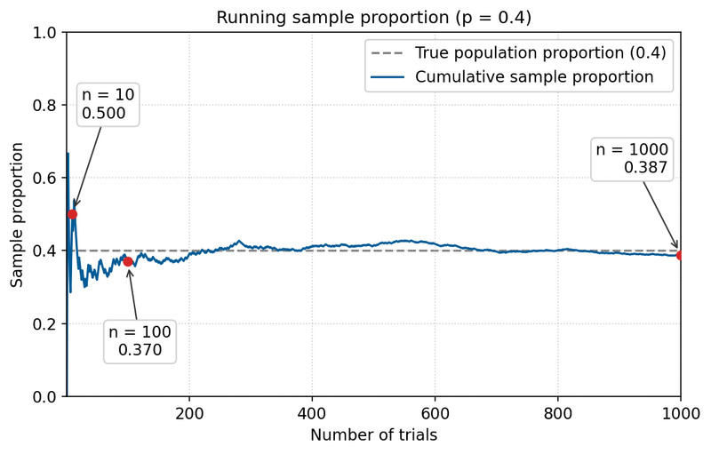
Running sample proportion approaching the true value (p = 0.4)

At first, the sample proportion swings wildly. With only a few trials, it even jumps above 0.60. By 100 trials it’s closer, and by 1000 trials it’s hovering right around the true proportion of 0.4. As the number of observations grows, the proportion stabilizes near the true value.

Important clarifications:

• It does not mean results will be exactly equal to expected.
• It does not remove randomness.
• It says long-run behavior becomes more stable.

So if you take a very large sample and still see a big difference from expected, that’s meaningful.

Preview of the p-value Idea

When we formally test whether results are unexpected, we calculate a p-value.

The p-value is:

The probability of getting results as extreme as (or more extreme than) what we observed, assuming the claim is true.

• Small p-value → Results would be rare if the claim were true → Evidence against the claim.
• Large p-value → Results are plausible under the claim → Not enough evidence to reject it.

Careful wording matters. The p-value is not:

• The probability the claim is true.
• The probability the results happened “by chance” without conditions.

It’s always conditional on the assumption that the claim is true.