Topic 4.2 Notes – Estimating Probabilities Using Simulation

1. Random Processes, Outcomes, and Events

A random process produces results determined by chance. You can’t predict one specific result, but you can describe long-run behavior.

Examples:

• Flipping a coin
• Selecting a student at random
• Using a random number generator

A trial is one repetition of that process.

An outcome is the result of a single trial.

• Rolling a 4 on a die
• Getting “Yes” on a survey

An event is a collection of one or more outcomes.

Here’s a concrete example with two dice. When you roll both dice once, the outcome is an ordered pair $(\text{Die 1}, \text{Die 2})$:

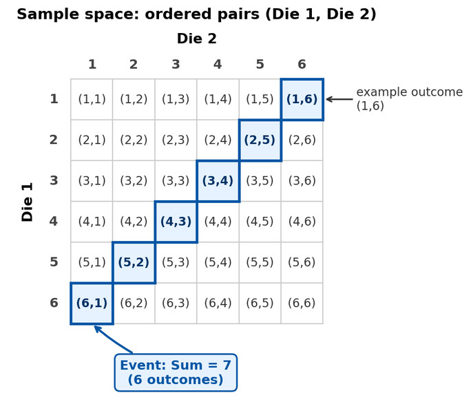
Sample space for two dice with the event “sum = 7” highlighted

Each ordered pair in the grid is an outcome.
The six highlighted ordered pairs together form the event “sum equals 7.”

Quick grounding:

• Probability is a number from 0 to 1.
• In the long run, probability ≈ proportion of times the event occurs.

Students often mix this up:

• Outcome = one specific result.
• Event = a set of outcomes.
• Trials are repeated; events are counted across trials.

That idea of long-run proportion is what makes simulation work.

2. What a Simulation Is and Why It Works

A simulation models a real random process using a chance device so the simulated outcomes behave like real ones.

The key requirement is this:
Your simulation must match the actual probability model.

If outcomes are equally likely → give them equal representation.
If probabilities differ → assign digits/regions proportionally.

Example: Suppose 30% of customers prefer Brand A and 70% prefer Brand B.
Using random digits:

• 0-2 → Brand A
• 3-9 → Brand B

That setup reflects 3 out of 10 digits for A, 7 out of 10 for B.

Simulation is especially useful when:

• The math is messy or complicated.
• There are many steps.
• You want a good estimate instead of an exact calculation.

If your model doesn’t match the real probabilities, your estimate will be biased. That’s one of the most common AP mistakes.

3. How to Design and Run a Simulation

On quizzes and FRQs, you must describe the simulation clearly enough that someone else could run it exactly as written.

Step 1: Describe One Trial

Be specific:

• What chance device are you using? (coins, dice, random digits, calculator)
• How does each outcome correspond to the real situation?
• What counts as a success?
• What do you record at the end of the trial?

If you skip any of these, you lose points.

Step 2: Repeat Many Trials

Run the simulation a large number of times.
Record whether each trial is a success or not.
Keep a count of total successes.

Step 3: Estimate the Probability

Use relative frequency:

$$\text{Estimated probability} = \frac{\text{Number of successes}}{\text{Total trials}}$$

Example: If 186 successes occur in 500 trials,

$$\frac{186}{500} = 0.372$$

In context:
“The estimated probability that a randomly selected customer prefers Brand A is approximately 0.372.”

Always state it in context. The AP readers look for the actual variable and situation.

4. Relative Frequency and the Law of Large Numbers

The relative frequency of an event is

$$\frac{\text{Number of times event occurs}}{\text{Total trials}}$$

Simulation uses this to estimate probability.

Law of Large Numbers

As the number of trials increases, the simulated probability gets closer to the true probability.

Here’s what that looks like in a simulation where the true probability is 0.5:

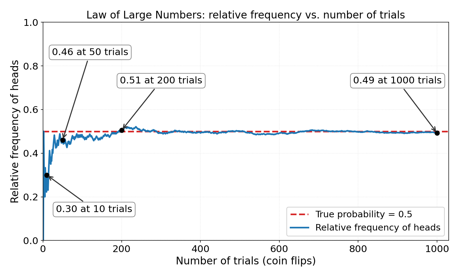
Running proportion of heads in 1,000 simulated coin flips: wide swings early, then a narrowing band around the true probability of 0.5

Early on, the graph jumps around and even drifts far from 0.5.
As trials increase, it settles in and fluctuates tightly around the true value.

Important:

• Short run = unpredictable.
• Long run = stable pattern.
• It does not guarantee quick “balancing out.”

Students often think things must even out quickly. They don’t. The law describes long-run behavior only.

5. Common Errors and What Gets Points Taken Off

• Not matching probabilities correctly in the model.
• Failing to define what counts as a success.
• Saying “repeat many times” without explaining how.
• Using very few trials.
• Claiming the simulated probability is the exact true probability.
• Forgetting to interpret the final proportion in context.

When graders read your response, they look for a clear trial description and a correct connection between simulation results and probability.