Topic 4.7 Notes – Introduction to Random Variables and Probability Distributions

1. What a Random Variable Is

A random variable (usually capital letters like $X$ or $Y$) assigns a numerical value to the outcome of a random process.

Think of it as a rule:

• Roll two dice → $X =$ sum of the two dice
• Survey a randomly selected family → $X =$ number of children
• Randomly select a litter → $X =$ number of puppies

The key idea:
The values of a random variable are the numerical outcomes of random behavior.

Discrete vs Continuous

You need to know the difference, even though this topic focuses on discrete.

Discrete random variable

• Takes a finite or countably infinite set of values (0, 1, 2, 3, …)
• Each value has its own probability
• Example: number of text messages received in an hour

Continuous random variable

• Can take any value in an interval
• Probabilities are assigned to intervals, not individual numbers
• Example: height, time, weight
  (Density curves and PDFs come later.)

One rule that always applies:

$$\sum P(X = x) = 1$$

All possible outcomes together must account for 100% of the probability.

2. Representing a Discrete Probability Distribution

A probability distribution lists:

• All possible values of $X$
• The probability for each value

Requirements for Validity

For a valid distribution:

1. $0 \le P(X = x) \le 1$
2. $\sum P(X = x) = 1$

If the probabilities add to 1.08 or include a negative number, it’s invalid. That’s an easy quiz point.

Common Representations

1. Table

Example: $X =$ number of correct answers on 3 true/false questions.

Each value has a probability. The probabilities add to 1, so this is a valid distribution.

2. Probability Histogram

The same distribution can be shown visually:

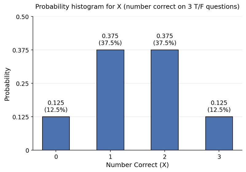
Probability histogram for number correct on 3 true/false questions

Each bar corresponds to one possible value of $X$. The bar heights match the probabilities from the table.

• Bars are separate because $X$ is discrete.
• The total of all bar heights is 1.

3. Function Notation

You’ll also see:

$$P(X = x)$$

This simply means “the probability that the random variable equals x.”

Cumulative Probability Distribution

Sometimes we want:

$$P(X \le x)$$

This is the cumulative probability.

Example:

• $P(X \le 2)$ = $P(0) + P(1) + P(2)$

Cumulative probabilities:

• Always increase
• Always end at 1

They can be shown in a table or as a function.

3. Finding Probabilities from a Distribution

Once the distribution is given, you answer questions by adding the correct probabilities.

Exact Value

$$P(X = 2)$$

Just read it from the table.

Interpreting Common Phrases

These show up constantly.

• At least k → $P(X \ge k)$ → include k
• At most k → $P(X \le k)$ → include k
• More than k → $P(X > k)$ → exclude k
• Less than k → $P(X < k)$ → exclude k

If wording feels tricky, list all possible values and circle the ones that qualify.

Using Complements

Often easier:

$$P(X \ge k) = 1 - P(X < k)$$

If “at least 4” means adding 4, 5, 6, 7, 8, it’s faster to subtract the lower values from 1.

This saves time on MCQs and reduces arithmetic mistakes.

4. Interpreting a Probability Distribution

On free-response, you must describe what the distribution tells you about the population.

Shape

From a histogram, describe:

• Symmetric
• Right-skewed
• Left-skewed
• Unimodal
• Bimodal

Always in context.

Example:
“The distribution of the number of puppies per litter is right-skewed, meaning smaller litters are more common but occasionally very large litters occur.”

Center

The mean is the long-run average value of the random variable.

Interpret like this:

“In the long run, we expect an average of 4.2 puppies per litter for this breed.”

It describes what would happen over many repetitions of the random process.

Spread

The standard deviation measures how far values typically vary from the mean.

• Larger SD → more variability
• Smaller SD → more consistency

Again, interpret in context of the variable.

5. Common Mistakes

• Forgetting probabilities must sum to 1.
• Mixing up discrete and continuous variables.
• Leaving out the boundary value for “at least” or “at most.”
• Describing shape without mentioning the variable or population.
• Saying “there is a probability the distribution is…” The distribution is fixed; it models behavior.