Topic 5.1 Notes – Introducing Statistics: Why Is My Sample Not Like Yours?

What a Sampling Distribution Is

Imagine repeatedly taking random samples of the same size $n$ from one population and calculating a statistic each time.

• Each sample gives you a value like:
  • Sample mean $\bar{x}$
  • Sample proportion $\hat{p}$
• If you recorded all those statistics, they would form a distribution.

That distribution is the sampling distribution.

So instead of a distribution of people, you now have a distribution of statistics.

Here’s the key shift:

• The population has one fixed mean $\mu$.
• Your samples produce many different $\bar{x}$ values.

Those different $\bar{x}$’s form a distribution. The histogram below shows what that looks like when many sample means (with $n = 5$) are collected.

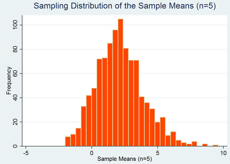
Sampling distribution of sample means (n = 5)

Even if every sample is random and done correctly, the sample means are not identical. That natural fluctuation is called sampling variability.

Parameters vs. Statistics

This distinction shows up constantly on quizzes and FRQs.

Population Parameters (fixed, usually unknown)

• Mean → $\mu$
• Standard deviation → $\sigma$
• Proportion → $p$

These describe the entire population. They do not change unless the population changes.

Sample Statistics (vary from sample to sample)

• Mean → $\bar{x}$
• Standard deviation → $s$
• Proportion → $\hat{p}$

These are calculated from a sample and change depending on which individuals were selected.

If a question says:

• “In a random sample of 120 voters…” → you are dealing with a statistic.
• “The true proportion of all registered voters…” → that’s a parameter.

The whole reason we study sampling distributions is because statistics vary. If they didn’t, we wouldn’t need inference.

Why My Sample Is Not Like Yours

Two students take random samples of 50 students from the same school and estimate the average number of hours of sleep. They get 6.8 hours and 7.3 hours.

Nobody did anything wrong.

This difference can happen because of random sampling variability.

Random Variation (expected)

Even with:

• Random selection
• Same population
• Same sample size

Statistics will differ.

That variation:

• Is unavoidable
• Follows patterns we can model
• Is the foundation of confidence intervals and hypothesis tests later

On AP questions, don’t say “the study must be flawed” just because two sample results differ. Variation alone is not evidence of bias.

Nonrandom Variation (problematic)

Sometimes differences happen because of:

• Undercoverage
• Nonresponse
• Convenience sampling
• Poor measurement

Now the variation is not just chance. It suggests bias or a design issue.

A good statistical thinker immediately asks:

• Is this difference explainable by random chance?
• Or is something wrong with how the data were collected?

That question drives everything in Unit 6 and beyond.

Statistics as Random Variables

A statistic like $\bar{x}$ is actually a random variable because its value depends on which sample you get.

Two types you should remember:

Discrete Random Variables

• Take countable values
• Example: number of defective items in a sample
• Displayed with a bar graph

Continuous Random Variables

• Can take any value in an interval
• Example: sample mean weight
• Displayed with a histogram or density curve

Here’s the visual difference. Discrete random variables have separate bars for each possible value. Continuous random variables are shown with a smooth curve.

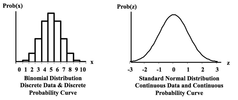
Discrete vs. continuous probability distributions

Sampling distributions for means and proportions are typically treated as continuous when $n$ is reasonably large.

Like any distribution, a sampling distribution has:

• Center
• Spread
• Shape

Later, you’ll learn how to calculate those precisely.

What Variation Should Make You Ask

Whenever you see different statistics from the same population, train yourself to ask:

1. How much variability is normal for this sample size?
2. Would a larger sample reduce the variability?
3. Is the difference larger than we’d expect by chance?
4. Could bias explain it instead?

The big idea of this topic:

Statistics vary.
Some variation is random and expected.
Because of that, conclusions are uncertain.

Inference is about deciding whether the variation you see is just random chance or evidence of something real.