Topic 8.3 Notes – Carrying Out a Chi-Square Test for Goodness of Fit

1. The Chi-Square Test Statistic for Goodness of Fit

A chi-square goodness of fit test compares:

• Observed counts (O) from your sample
• Expected counts (E) based on a claimed population distribution (your null model)

The test statistic is:

$$\chi^2 = \sum \frac{(O - E)^2}{E}$$

Where:

• $O$ = observed count in a category
• $E$ = expected count in that category
• You add up the value for all categories.

What each part is doing

Each term $\frac{(O - E)^2}{E}$:

• Measures how far one category’s data is from what was predicted.
• Squaring makes all differences positive.
• Dividing by $E$ adjusts for category size. A difference of 10 matters more if you expected 20 than if you expected 500.

Because everything is squared, χ² is always 0 or larger.

• χ² near 0 → observed counts are close to expected → supports $H_0$
• Large χ² → big differences → evidence against $H_0$

Degrees of freedom

$$df = \text{number of categories} - 1$$

If you have 5 categories, then $df = 4$.

What the null distribution looks like

If the null hypothesis (and its probability model) is true, the test statistic follows a chi-square distribution with the appropriate $df$.

Here are several chi-square distributions for different degrees of freedom.

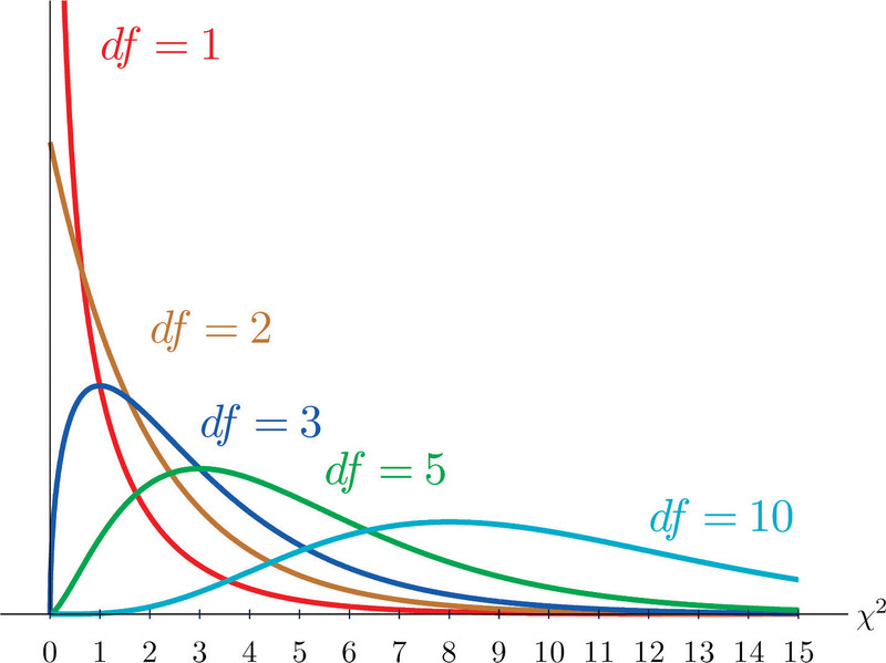
Chi-square distributions for different degrees of freedom

Key features:

• Only defined for values ≥ 0
• Right-skewed
• Larger $df$ → more spread out and more symmetric

As $df$ increases, the curve shifts to the right and becomes less skewed, but it always stays nonnegative and right-skewed.

In some settings, a randomization distribution could be used instead of the theoretical chi-square curve, but on the AP exam you’ll almost always use the chi-square distribution.

2. Calculating the Chi-Square Statistic

Here’s what this looks like in action.

Imagine a company claims customer preferences are:

• 50% Product A
• 30% Product B
• 20% Product C

You survey 200 customers and observe:

• A: 88
• B: 74
• C: 38

Step-by-step

1. Find expected counts

   $$E = n \times p_0$$

   • A: $200 \times 0.50 = 100$
   • B: $200 \times 0.30 = 60$
   • C: $200 \times 0.20 = 40$

2. Compute each component

   $$\chi^2 = \frac{(88-100)^2}{100} + \frac{(74-60)^2}{60} + \frac{(38-40)^2}{40}$$

   $$= \frac{144}{100} + \frac{196}{60} + \frac{4}{40}$$

   $$= 1.44 + 3.27 + 0.10 = 4.81$$

3. Degrees of freedom

   $$df = 3 - 1 = 2$$

Using technology

On a calculator: use χ²GOF-Test, enter:

• Observed list
• Expected list

It gives you χ², $df$, and the p-value.

Common mistakes I see every year:

• Plugging in proportions instead of counts
• Forgetting to square
• Using the wrong $df$

3. Finding and Interpreting the p-Value

Once you have χ² and $df$, the p-value is:

The probability, assuming the null hypothesis and its probability model are true, of getting a chi-square statistic as large or larger than the one observed.

Because the chi-square distribution is right-skewed:

• The p-value is the area to the right of your χ² value.

Large χ² → small p-value → stronger evidence against $H_0$.

You can:

• Use calculator output (best option), or
• Use a chi-square table with the correct $df$.

Interpreting the p-value in context

Your interpretation must include:

• “Assuming the null hypothesis is true”
• The test statistic (or “a chi-square statistic”)
• The numeric p-value
• The real-world context

Example:

If the company’s claimed distribution is correct, the probability of getting a chi-square statistic of 4.81 or larger from a sample of 200 customers is 0.09.

Never say:

• “There is a 9% chance the null is true.”
• “There is a 9% chance the results happened by chance.”

4. Making a Decision and Stating the Conclusion

Compare the p-value to your significance level $\alpha$.

• If p ≤ α → Reject $H_0$
• If p > α → Fail to reject $H_0$

Never say “accept $H_0$.”

Writing the conclusion

You need:

1. Decision
2. “Convincing evidence”
3. Population + variable in context

If p = 0.09 and α = 0.05:

Since 0.09 > 0.05, we fail to reject the null hypothesis. There is not convincing evidence that the true distribution of customer preferences differs from the company’s claimed distribution.

Big picture meaning:

• A significant result means at least one category proportion is different.
• The test does not tell you which one.
• A non-significant result means the data are consistent with the claimed distribution, not that it’s proven correct.