Topic 5.4 Notes – Biased and Unbiased Point Estimates

1. What a Point Estimator Is

Start with the language. You have to keep these straight:

• A parameter describes a population
  • $\mu$ = population mean
  • $p$ = population proportion
  • $\sigma$ = population standard deviation
• A statistic describes a sample
  • $\bar{x}$ = sample mean
  • $\hat{p}$ = sample proportion
  • $s$ = sample standard deviation

A point estimate is a single number from your sample that estimates a population parameter.

A point estimator is the rule or formula used to compute that number from sample data.

Examples you should automatically know:

• $\bar{x}$ is a point estimator of $\mu$
• $\hat{p}$ is a point estimator of $p$
• $s$ is a point estimator of $\sigma$

Here’s the key idea that ties Unit 5 together:

Because different random samples give different values of $\bar{x}$ or $\hat{p}$, a point estimator is a random variable.

That means it has a sampling distribution with:

• A mean (which tells us about bias)
• A standard deviation (which tells us about variability)

That’s where this topic lives.

2. What It Means for an Estimator to Be Unbiased

An estimator is unbiased if the mean of its sampling distribution equals the true population parameter.

In symbols:

• $\bar{x}$ is unbiased for $\mu$ if
  $$\text{mean of the sampling distribution of } \bar{x} = \mu$$
• $\hat{p}$ is unbiased for $p$ if
  $$\text{mean of the sampling distribution of } \hat{p} = p$$

What this means in plain language:

If you repeatedly take many random samples and compute the statistic each time, the average of all those statistics will equal the true parameter.

Individual samples will be too high or too low. That’s normal. Bias is about the long-run center, not one result.

Visualizing unbiased vs biased

Think about where the sampling distribution is centered.

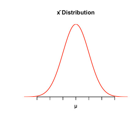
Sampling distribution of $\bar{x}$ centered at $\mu$

In this diagram, the peak of the sampling distribution lines up with $\mu$. That alignment is what makes an estimator unbiased.

If the entire distribution were shifted left or right so its center did not match $\mu$, the estimator would be biased.

Notice this is about the center, not the spread.

3. Bias vs Variability

Students mix these up every year. They are different properties.

Bias and accuracy

• Is the sampling distribution centered at the true parameter?
• If yes → unbiased.
• If consistently above or below → biased.
• Increasing sample size does not fix bias from a flawed method.

Bias is about location.

Variability = Consistency

• How spread out is the sampling distribution?
• Measured by the standard deviation of the sampling distribution (the standard error).
• Larger $n$ → smaller variability.
• Zero variability is impossible because of sampling error.

Variability is about spread.

The bullseye picture

This classic target diagram ties it all together. The center represents the true parameter. The blue dots represent estimates from many repeated samples.

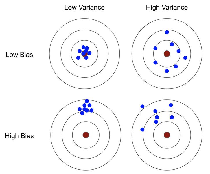
Bias and variability illustrated with target diagrams

• Tight and centered → best case.
• Tight but off-center → biased but consistent.
• Spread but centered → unbiased but high variability.
• Spread and off-center → worst case.

On tests, if they describe “estimates that are consistently too high,” that’s bias.
If they describe “estimates that vary a lot from sample to sample,” that’s variability.

4. How to Determine If an Estimator Is Biased

When you’re asked to explain whether something is unbiased, think in this order.

Step 1: Identify the parameter and estimator

Example:
Parameter = true proportion of voters who support a policy.
Estimator = $\hat{p}$, the sample proportion from a survey.

Be specific.

Step 2: Think about repeated sampling

Ask yourself:

If we repeatedly took random samples and calculated this statistic each time, where would its sampling distribution be centered?

If centered at the true parameter → unbiased.

That’s the reasoning the AP rubric wants.

Step 3: Consider how the data were collected

Important distinction:

• $\bar{x}$ is theoretically an unbiased estimator of $\mu$.
• But a nonrandom sample, undercoverage, nonresponse, or voluntary response can produce biased estimates in practice.

The formula may be unbiased. The method might not be.

This shows up often in free response. They’ll describe a flawed survey and ask if the estimator is unbiased. You need to connect bias to the sampling process.

5. Common Mistakes and Exam Traps

• One sample mean not equal to $\mu$ does not prove bias. Bias is long-run.
• Don’t say “the sample is unbiased.” Say “the estimator is unbiased.”
• Large sample size reduces variability, not bias from poor design.
• Always tie your explanation to the idea of the mean of the sampling distribution.