Topic 5.5 Notes – Sampling Distributions for Sample Proportions

What a Sampling Distribution of p̂ Is

When you take one random sample from a population and calculate a sample proportion,

$$\hat{p} = \frac{\text{number of successes}}{n},$$

that’s just one number.

Now imagine taking many independent random samples of the same size $n$ from the same population and calculating $\hat{p}$ each time. The distribution of all those possible $\hat{p}$ values is the sampling distribution of $\hat{p}$.

Important distinction:

• The original data are categorical (success/failure).
• The random variable in this topic is the proportion $\hat{p}$.
• The population proportion $p$ is fixed.
• The sample proportion $\hat{p}$ varies from sample to sample.

Here’s what that idea looks like visually. A population with $p = 0.40$ leads to different sample proportions like 0.36, 0.39, and 0.42, and those values form a distribution centered at 0.40.

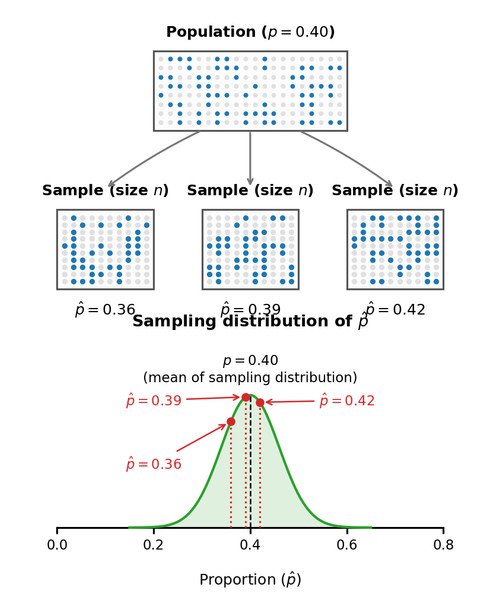
From population proportion to sampling distribution of $\hat{p}$

Even though individual responses are 0 or 1, the distribution of $\hat{p}$ follows predictable probability rules. That’s the big idea.

Mean and Standard Deviation of p̂

Assume independent sampling (either sampling with replacement or sampling without replacement but meeting the 10% condition).

Mean

$$\mu_{\hat{p}} = p$$

The sampling distribution is centered at the true population proportion.

This means $\hat{p}$ is an unbiased estimator of $p$. On average, sample proportions land at the true value.

Standard Deviation

$$\sigma_{\hat{p}} = \sqrt{\frac{p(1-p)}{n}}$$

This tells you how much $\hat{p}$ typically varies from sample to sample.

What affects it?

• Larger $n$ → smaller standard deviation → less variability
• When $p = 0.5$, variability is largest
• As $p$ gets closer to 0 or 1, variability shrinks

In context, you would say:

The standard deviation of the sample proportion is 0.03, meaning sample proportions typically differ from the true population proportion by about 0.03.

Notice the units are proportions, not individuals.

Sampling Without Replacement and the 10% Condition

If sampling without replacement, the true standard deviation is slightly smaller than the formula above.

We ignore that difference if:

$$n < 10\% \text{ of the population size}$$

This is the 10% condition, and it lets us treat observations as approximately independent.

Students often forget this condition on quizzes. If the population size is given, check it.

When the Sampling Distribution Is Approximately Normal

Even though the data are categorical, the distribution of $\hat{p}$ can look normal if the sample is large enough.

Large Counts Condition

We need:

$$np \ge 10 \quad \text{and} \quad n(1-p) \ge 10$$

Both the expected number of successes and failures must be at least 10.

If this condition is met:

• Shape ≈ Normal
• Center = $p$
• Spread = $\sqrt{\frac{p(1-p)}{n}}$

The grid below shows sampling distributions of $\hat{p}$ for different values of $p$ (rows) and increasing sample sizes $n$ (columns). As you move to the right, the distributions become more symmetric and bell-shaped.

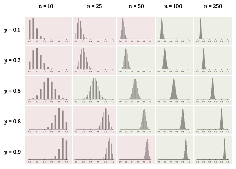
Sampling distributions of $\hat{p}$ for different values of $p$ and $n$

When $n$ is small or when $p$ is close to 0 or 1, the distributions are skewed. As $n$ increases and the large counts condition is satisfied, the shape becomes approximately normal.

Common issue: Students say “n is large” without checking $np$ and $n(1-p)$. For proportions, you must check both.

Interpreting Probabilities About p̂

When the distribution is approximately normal, we can compute probabilities using z-scores.

The standardized value is:

$$z = \frac{\hat{p} - p}{\sigma_{\hat{p}}}$$

Important:

• We calculate probabilities about $\hat{p}$.
• The population proportion $p$ does not change.

Example of interpretation:

The probability that the sample proportion of voters who support the policy is greater than 0.55 is 0.08. This means that in repeated random samples of size 200, about 8% of sample proportions would exceed 0.55.

Always mention:

• The population
• The sample size
• That we’re talking about repeated random samples

That’s exactly how AP graders want it phrased.