Topic 5.8 Notes – Sampling Distributions for Differences in Sample Means

1. The Sampling Distribution of $\bar{x}_1 - \bar{x}_2$

Picture this: you randomly sample students from School A and School B, compute each sample’s mean test score, and subtract. If you repeated that process over and over, each time calculating

$$\bar{x}_1 - \bar{x}_2,$$

those values would form a sampling distribution.

Assume:

• Population 1: mean $\mu_1$, standard deviation $\sigma_1$, sample size $n_1$
• Population 2: mean $\mu_2$, standard deviation $\sigma_2$, sample size $n_2$
• Samples are random and independent

Mean and Standard Deviation

The sampling distribution has predictable parameters:

$$\mu_{\bar{x}_1 - \bar{x}_2} = \mu_1 - \mu_2$$

The average of all possible sample differences equals the true population difference. That’s why $\bar{x}_1 - \bar{x}_2$ is an unbiased estimator of $\mu_1 - \mu_2$.

$$\sigma_{\bar{x}_1 - \bar{x}_2} = \sqrt{\frac{\sigma_1^2}{n_1} + \frac{\sigma_2^2}{n_2}}$$

Important details:

• You add variances, not standard deviations.
• Larger sample sizes make the distribution less spread out.
• More variability in either population increases the spread.

Students often forget to square the standard deviations before dividing by sample size. That mistake costs easy points.

2. Shape of the Sampling Distribution

Now we care about when this distribution is normal (or approximately normal), because that’s what lets us calculate probabilities using z-scores.

If Both Populations Are Normal

If each population distribution is normal, then $\bar{x}_1 - \bar{x}_2$ is exactly normal, no matter the sample sizes.

If Populations Are Not Normal

This is where the Central Limit Theorem kicks in.

If both sample sizes are at least 30:

• Each sample mean is approximately normal.
• The difference of two approximately normal distributions is also approximately normal.

So we can model $\bar{x}_1 - \bar{x}_2$ as normal.

Here’s the idea visually. The left panel shows a heavily skewed population. As the sample size increases (middle and right panels), the sampling distribution of the mean becomes more bell-shaped.

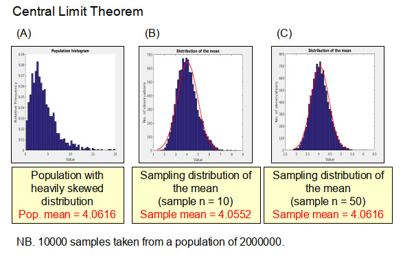
Central Limit Theorem illustration

On tests, you must justify normality for both groups. If one sample is large and the other is small from a skewed population, you cannot assume normality.

3. Sampling With and Without Replacement

The standard deviation formula technically assumes sampling with replacement.

If sampling without replacement:

• The true standard deviation is slightly smaller.
• If each sample size is less than 10% of its population, the difference is negligible.

This is the familiar 10% condition. On the AP exam, you state it to justify independence when sampling from a large population without replacement.

If the two samples come from completely separate populations, they’re automatically independent.

4. Using the Distribution to Find Probabilities

Suppose:

• $\mu_1 = 82$, $\sigma_1 = 10$, $n_1 = 40$
• $\mu_2 = 78$, $\sigma_2 = 12$, $n_2 = 50$

First find the parameters:

$$\mu_{\bar{x}_1 - \bar{x}_2} = 82 - 78 = 4$$

$$\sigma_{\bar{x}_1 - \bar{x}_2} = \sqrt{\frac{10^2}{40} + \frac{12^2}{50}} = \sqrt{\frac{100}{40} + \frac{144}{50}} = \sqrt{2.5 + 2.88} = \sqrt{5.38} \approx 2.32$$

If we want $P(\bar{x}_1 - \bar{x}_2 > 6)$:

$$z = \frac{6 - 4}{2.32} \approx 0.86$$

Then use the normal table or calculator.

Interpretation in context matters. For example:

The mean of the sampling distribution is 4 points, meaning that in repeated sampling, the average difference in sample mean scores (School A minus School B) would be 4 points. The standard deviation is about 2.32 points, meaning the difference in sample means typically varies by about 2.32 points from sample to sample.

Units always stay attached.

5. Common Mistakes

• Subtracting standard deviations instead of adding variances.
• Checking the CLT condition for only one sample.
• Forgetting to mention independence or the 10% condition.
• Using this formula for paired data. Paired means use a different approach.
• Giving probability answers without context or units.