Topic 1.9 Notes – Comparing Distributions of a Quantitative Variable

1. What It Means to Compare Distributions

When you compare independent samples (like test scores from two classes or commute times in two cities), you are comparing their entire distributions, not just single numbers.

Every comparison should revolve around the same four features:

• Shape
  Skewed left or right? Symmetric? One peak or more than one?
• Center
  Median or mean. Where is the “typical” value?
• Spread
  IQR, range, or standard deviation. How variable are the values?
• Unusual features
  Outliers, gaps, clusters.

The key is direct comparison language. Not “Class A has a median of 78. Class B has a median of 72.”
Instead:

“Class A has a higher median test score than Class B.”

On quizzes and the AP exam, points are lost when students describe groups separately instead of comparing them.

2. Comparing Graphical Displays

Any appropriate graph works as long as it allows you to compare:

• Histograms (with same scale)
• Dotplots
• Stem-and-leaf plots
• Side-by-side boxplots

Here’s what side-by-side boxplots look like when comparing two groups:

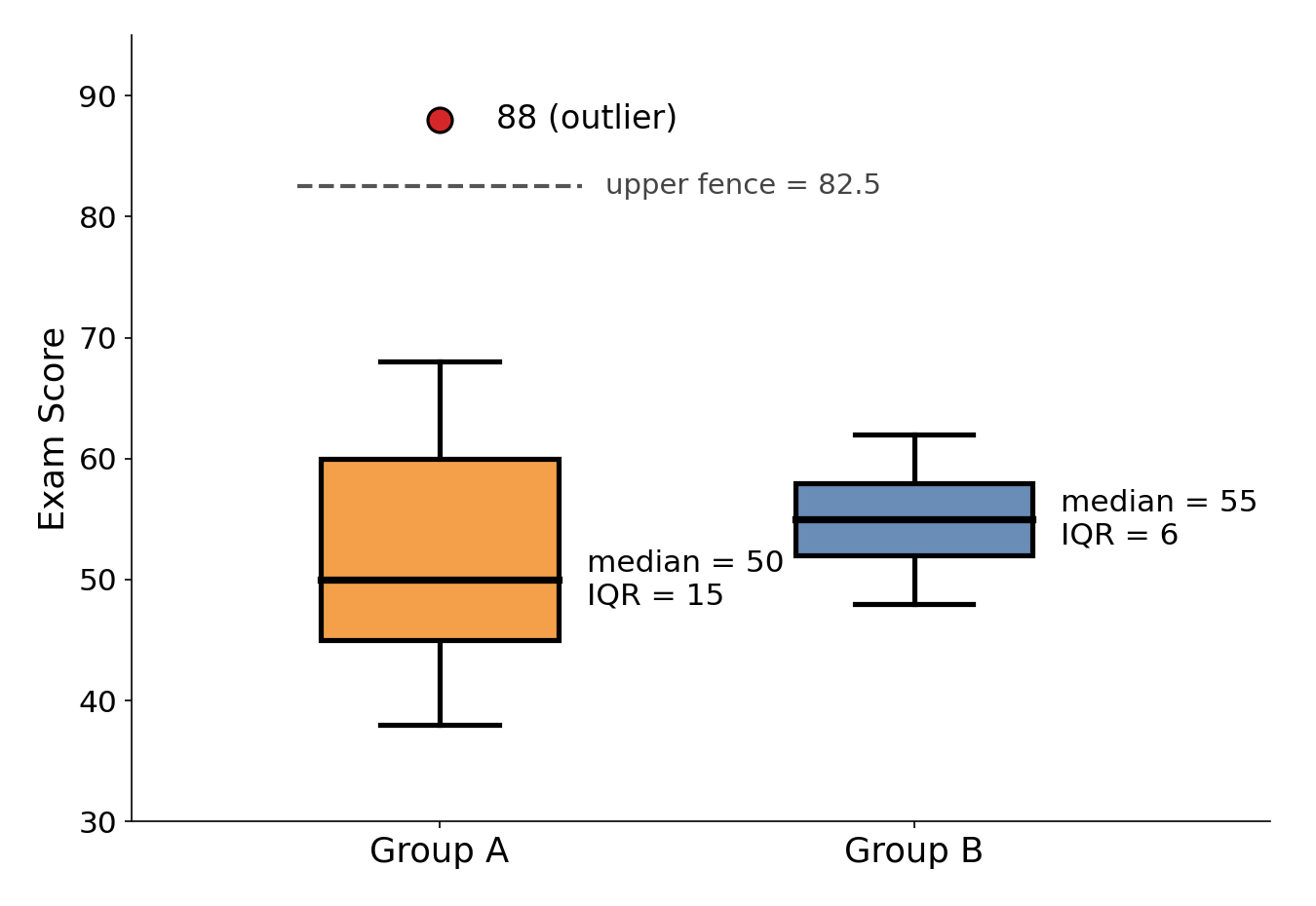
Side-by-side boxplots comparing exam scores for Group A and Group B. Group A's upper fence is $Q_3 + 1.5 \times \text{IQR} = 60 + 1.5(15) = 82.5$, so the score of 88 is an outlier.

Notice that one group has a high outlier and a wider box, while the other is more tightly clustered. That is exactly the kind of visual information you are expected to describe.

Shape

Look for:

• Skewness
  • Right-skewed → long tail to the right
  • Left-skewed → long tail to the left
• Modality (one peak or multiple)

In the boxplots above, one distribution is right-skewed because of a high outlier.

Shape matters because it affects how you interpret center:

• In right-skewed data, the mean is pulled higher than the median.
• In left-skewed data, the mean is pulled lower than the median.

If shapes differ, mention it clearly.

Center

Use:

• Median for skewed data or boxplots.
• Mean for roughly symmetric data without strong outliers.

From the boxplots above, you would compare the medians to describe which group has the higher typical score.

When estimating from a histogram:

• The median splits the area in half.
• For even $n$, it falls between the two middle observations.

Always state comparisons in context:

“The median commute time for City A residents is higher than that of City B residents.”

Spread

Ways to compare variability:

• Range = max − min
• IQR = $Q_3 - Q_1$
• Standard deviation (spread around the mean)

Bigger spread means more variability.

In the boxplots above, the group with the wider box has the larger IQR, so its middle 50% of scores are more spread out.

Be specific:

• “Group A has a larger IQR, so the middle 50% of its values are more spread out.”
• “Group B’s scores are more tightly clustered.”

Spread should be compared relative to center, not just extremes.

Unusual Features

Look for:

• Outliers (shown as dots on boxplots)
• Gaps in histograms
• Clusters of values

Outliers especially matter because they:

• Strongly affect the mean
• Increase the standard deviation

The boxplots above show a high outlier in one group, which would pull its mean upward and increase its standard deviation.

If you see one, mention it and explain how it affects interpretation.

3. Comparing Numerical Summary Statistics

Sometimes you won’t see a graph. You’ll just get numbers:

• Means
• Medians
• Standard deviations
• IQRs
• Ranges

You still compare center and variability directly.

Comparing Centers

• Higher mean → larger average value
• Higher median → larger typical value

If one distribution is skewed and the other is symmetric, the mean may not be the best measure for both. In skewed data, the median is more reliable.

Comparing Variability

• Larger standard deviation → more spread around the mean
• Larger IQR → more spread in the middle 50%
• Larger range → wider overall spread

Remember: standard deviation measures typical distance from the mean, not total width.

4. Writing a Strong Comparison

A complete comparison usually follows this flow:

1. Compare shape
2. Compare center
3. Compare spread
4. Mention unusual features
5. Use context

Example:

“Both distributions of daily screen time are unimodal, but teens are more right-skewed than adults. The median screen time for teens is higher than for adults, indicating a higher typical number of hours per day. Teens also show greater variability, with a larger IQR and range. There is a high outlier among teens that may increase the mean screen time.”

Common issues that cost points:

• Forgetting to mention spread
• Ignoring shape
• Not writing in context
• Claiming causation when you’re only comparing