Topic 9.5 Notes – Carrying Out a Test for the Slope of a Regression Model

1. The Slope Test in Linear Regression

In simple linear regression, we model the relationship between an explanatory variable $x$ and a response variable $y$:

$$y = \beta_0 + \beta_1 x + \varepsilon$$

• $\beta_1$ = true population slope
• $b$ = sample slope from the least-squares regression line (estimate of $\beta_1$)

A test for the slope asks whether the true slope $\beta_1$ differs from some value (almost always 0).

Most common hypotheses:

• H₀: $\beta_1 = 0$
  (No linear relationship in the population.)
• Hₐ:
  • $\beta_1 \ne 0$ (two-sided)
  • $\beta_1 > 0$
  • $\beta_1 < 0$

If $\beta_1 = 0$, changes in $x$ do not predict changes in the mean of $y$.

When conditions are met and $H_0$ is true, the slope statistic follows a t-distribution. That’s the key idea of this whole topic.

2. Conditions and the Null Distribution of the Slope

Before doing any calculations, regression inference requires the LINE conditions:

• Linear: The relationship looks linear (check scatterplot and residual plot).
• Independent: Observations are independent (random sample or random assignment; 10% condition if sampling).
• Normal: For each value of $x$, the response is normally distributed (or sample is large).
• Equal variance: Residuals show constant spread (no funnel shape).

Here’s what violations look like in a residual plot. In the top two graphs the residuals stay centered on 0, but their spread grows (top) or shrinks (middle) as $x$ increases. That fan shape signals a problem with the equal variance condition. The bottom graph shows random scatter with roughly constant spread, which is what you want to see.

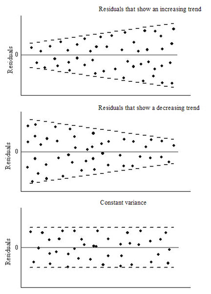
Residual plots: patterns vs. constant variance

If these conditions are satisfied and $H_0$ is true, then the standardized slope

$$t = \frac{b}{SE_b}$$

follows a t-distribution with df = n − 2.

Important pieces:

• $b$ = sample slope (estimate of $\beta_1$)
• Typical test: $H_0: \beta_1 = 0$, so $t = b/SE_b$ (same as $(b - 0)/SE_b$)
• $SE_b$ = standard error of the slope
• df = n − 2

Why $n - 2$? Because we estimated two parameters from the data: the intercept and the slope.

3. Calculating the Test Statistic and p-Value

Step 1: State hypotheses in context

Example wording:

Let $\beta_1$ be the true slope relating hours of sleep to reaction time for high school students.

Then state $H_0$ and $H_a$.

You must define $\beta_1$ in words. Skipping that costs points.

Step 2: Compute the test statistic

$$t = \frac{b}{SE_b}$$

This tells you how many standard errors your sample slope is from the hypothesized slope.

If $b = 1.8$, $SE_b = 0.6$, and testing $H_0: \beta_1 = 0$:

$$t = \frac{1.8 - 0}{0.6} = 3$$

That means the observed slope is 3 standard errors above 0.

Step 3: Find the p-value

Use:

• t-distribution
• df = $n - 2$
• One- or two-sided based on $H_a$

The p-value is:

The probability of getting a slope statistic at least as extreme as the one observed, assuming $H_0$ (for example $H_0: \beta_1 = 0$) is true.

Calculator note: Most regression output already gives you the t-value and p-value. Just be sure the df matches $n-2$.

4. Making and Justifying the Conclusion

Compare the p-value to $\alpha$:

• If $\text{p-value} \le \alpha$, reject $H_0$.
• If $\text{p-value} > \alpha$, fail to reject $H_0$.

Your conclusion must:

1. State the decision.
2. Answer the research question.
3. Refer to a linear relationship.
4. Stay in context.

Example (rejecting):

Since the p-value is less than 0.05, we reject $H_0$. There is convincing evidence of a linear relationship between hours of sleep and mean reaction time for high school students.

Notice it says linear and names both variables.

The test result is your statistical reasoning supporting the research claim.

5. Interpretation and Common Mistakes

Correct p-value interpretation

Always include the assumption:

Assuming $\beta_1 = 0$, the probability of obtaining a sample slope this extreme (or more extreme) is ___.

Students often forget the “assuming $H_0$ is true” part. That assumption is the entire logic of significance testing.

Common AP mistakes

• Using df = n − 1 instead of $n − 2$.
• Saying “there is a relationship” instead of “there is a linear relationship.”
• Claiming causation with observational data.
• Forgetting to define $\beta_1$.
• Saying the p-value is the probability that $H_0$ is true.

That last one shows up constantly on multiple choice.