Topic 4.8 Notes – Mean and Standard Deviation of Random Variables

1. Parameters of a Discrete Random Variable

A parameter is a single, fixed numerical value that describes a population or the distribution of a random variable.

When you’re given a discrete random variable $X$ (usually with a probability table), the two key parameters are:

• Mean $\mu_X$ → center
• Standard deviation $\sigma_X$ → spread

These describe the distribution of X itself, not a sample. Even though outcomes vary, the parameters are fixed numbers.

Important reminders:

• Both $\mu_X$ and $\sigma_X$ are in the same units as X.
• They describe long-run behavior if the chance process is repeated many times.
• They are not statistics like $\bar{x}$ or $s$. Those come from samples.

2. The Mean or Expected Value $\mu_X$

The mean of a discrete random variable is also called the expected value. Think of it as a weighted average, where probabilities act as weights.

Formula

$$\mu_X = \sum x_i \cdot P(X = x_i)$$

You multiply each possible value by its probability and add.

Here’s what that looks like with an actual probability distribution:

Expected value from a discrete probability distribution

What it means

• It’s the long-run average outcome.
• It may be a decimal even if X only takes whole numbers.
• It does not represent a probability.

Correct interpretation example:

In the long run, the average number of defective items per shipment is about 1.7 items.

Notice:

• It names the variable.
• It includes units.
• It uses long-run language.

Common mistakes I see on quizzes:

• Just averaging the x-values without using probabilities.
• Rounding to a whole number because “you can’t have 1.7 items.”
• Saying “There is a 1.7 probability…” which makes no sense.

3. Variance and Standard Deviation $\sigma_X$

Mean tells you center. Now we measure how spread out the distribution is.

Variance

$$\text{Var}(X) = \sum (x_i - \mu_X)^2 \cdot P(X = x_i)$$

This is the average squared distance from the mean.

Standard Deviation

$$\sigma_X = \sqrt{\sum (x_i - \mu_X)^2 \cdot P(X = x_i)}$$

This puts the measure back in the original units, which is why we interpret standard deviation, not variance.

Conceptually, you:

1. Subtract the mean from each value.
2. Square it.
3. Multiply by its probability.
4. Add.
5. Take the square root.

Here’s what different spreads look like when the mean stays the same:

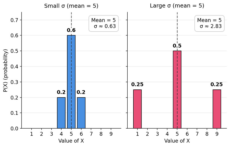
Two discrete distributions with the same mean but different standard deviations

Both distributions have mean 5. The one on the left is tightly clustered around 5, so its standard deviation is small. The one on the right puts more probability far from 5, so its standard deviation is larger.

Interpretation

Correct format:

The number of defective items per shipment typically varies by about 0.9 items from the mean of 1.7 items.

Key words:

• “typically”
• “from the mean”
• includes units

Students often lose points by writing:

• “The standard deviation is 0.9.” (No context.)
• Or forgetting to mention the mean.

4. Interpreting Parameters in Context

On tests and the AP exam, calculations alone don’t earn full credit. Your interpretation must:

• Refer to the random variable
• Include the units
• Use long-run or typical language

Mean → long-run average
Standard deviation → typical distance from the mean

If a question says “Describe the distribution,” they want both ideas: center and spread, stated in context.

5. Big Picture Connections

A probability distribution models population variation. The parameters $\mu_X$ and $\sigma_X$ summarize that variation.

Think of it this way:

• A histogram of data → summarized by $\bar{x}$ and $s$.
• A probability distribution → summarized by $\mu_X$ and $\sigma_X$.

Same ideas. Different setting.

Whenever you see a probability table, your brain should immediately think:

• Weighted average for the mean.
• Typical distance from the mean for spread.