Topic 5.6 Notes – Sampling Distributions for Differences in Sample Proportions

What the sampling distribution of $\hat p_1 - \hat p_2$ is

Imagine two independent populations:

• Population 1 has true proportion $p_1$
• Population 2 has true proportion $p_2$

We take:

• A random sample of size $n_1$ → compute $\hat p_1$
• A random sample of size $n_2$ → compute $\hat p_2$

Now we look at the statistic:

$$\hat p_1 - \hat p_2$$

If we repeated this whole process many times, those differences would form a sampling distribution.

Mean (Center)

$$\mu_{\hat p_1 - \hat p_2} = p_1 - p_2$$

The estimator is unbiased. On average, the sample difference equals the true population difference.

If the true difference is 0.08, the sampling distribution is centered at 0.08.

Standard Deviation (Spread)

$$\sigma_{\hat p_1 - \hat p_2} = \sqrt{ \frac{p_1(1-p_1)}{n_1} + \frac{p_2(1-p_2)}{n_2} }$$

Two key ideas are built into this formula:

• Each proportion has variability $\frac{p(1-p)}{n}$
• Variances add for independent samples

Students sometimes forget that you add the two variance pieces before taking the square root.

What affects the spread?

• Larger $n_1$ or $n_2$ → smaller spread
• Proportions near 0.5 → larger variability
• Proportions near 0 or 1 → smaller variability

If sampling without replacement, the true standard deviation is slightly smaller than the formula gives. As long as each sample is less than 10% of its population, the difference is negligible and we use the formula above.

When the distribution is approximately normal

The sampling distribution of $\hat p_1 - \hat p_2$ is approximately Normal when sample sizes are large enough.

1. Independent random samples

• Each sample is random (SRS or random assignment)
• The two samples are independent of each other

2. 10% condition (if sampling without replacement)

$$n_1 \le 0.10N_1 \qquad n_2 \le 0.10N_2$$

This supports the standard deviation formula.

3. Large Counts condition

All four must be true:

$$n_1 p_1 \ge 10$$

$$n_1(1-p_1) \ge 10$$

$$n_2 p_2 \ge 10$$

$$n_2(1-p_2) \ge 10$$

You are checking for enough expected successes and failures in both samples.

When these conditions are met, the sampling distribution looks like this:

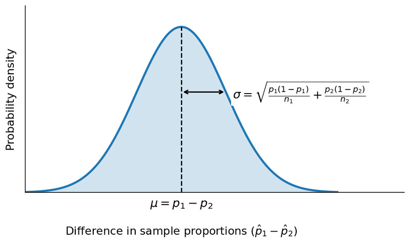
Normal model for $\hat p_1 - \hat p_2$

The curve is centered at $\mu = p_1 - p_2$ and has standard deviation $\sqrt{\frac{p_1(1-p_1)}{n_1} + \frac{p_2(1-p_2)}{n_2}}$, the formula you saw earlier.

Important detail: for proportions, we use the Large Counts condition, not the CLT for means. That distinction shows up in multiple-choice questions.

Shape, Center, and Spread Summary

When conditions are met:

• Shape: Approximately Normal
• Center: $p_1 - p_2$
• Spread: $\sqrt{\frac{p_1(1-p_1)}{n_1} + \frac{p_2(1-p_2)}{n_2}}$

If an FRQ asks you to “describe the sampling distribution,” you must state all three and justify normality using the Large Counts condition.

Interpreting parameters and probabilities in context

This is where points are often lost. Everything must reference:

• Random sampling
• Repeated samples
• The specific populations

Interpreting the mean

“The mean of the sampling distribution is $p_1 - p_2$, meaning that in repeated random samples, the average difference in sample proportions would equal the true difference in population proportions of [state the actual groups].”

Parameters are fixed. The sample statistic varies.

Interpreting the standard deviation

This describes typical sampling variability in the difference from sample to sample. It does not describe individual variability.

Interpreting a probability

If you compute something like

$$P(\hat p_1 - \hat p_2 > 0.05)$$

You would say:

“This is the probability that the difference in sample proportions would exceed 0.05 in repeated random samples from these two populations, assuming the stated population proportions are correct.”

You are describing long-run behavior of the statistic.