Topic 2.7 Notes – Residuals

1. What a Residual Is and What It Tells You

A residual measures how far a single data point is from what the regression line predicted.

The formula is:

$$\text{residual} = y - \hat{y}$$

• $y$ = actual (observed) response
• $\hat{y}$ = predicted response from the LSRL

So a residual is just actual minus predicted.

What it represents visually

A residual is the vertical distance from a point to the regression line.

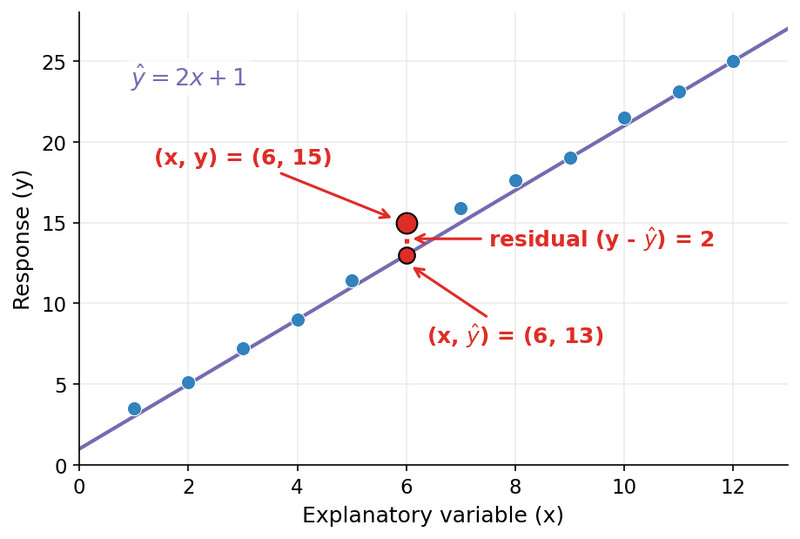
Residual shown as vertical distance from a point to the LSRL

In the graph, the observed point is above the line, so the vertical segment from the line up to the point is the residual.

Notice it’s vertical, not diagonal. We measure how far up or down the point is from the line.

Sign of a residual

• Positive residual → $y > \hat{y}$
  The model underestimates the actual value.
• Negative residual → $y < \hat{y}$
  The model overestimates the actual value.
• Residual = 0 → the point lies exactly on the line.

The least squares regression line is chosen to minimize the sum of the squared residuals. That’s where the name “least squares” comes from.

Small residual → good prediction for that point.
Large residual → poor prediction.

2. How to Calculate and Interpret a Residual

You’ll often be given a regression equation and asked for a residual.

Step-by-step

1. Plug the x-value into the regression equation to find $\hat{y}$.
2. Subtract: $\text{residual} = y - \hat{y}$.
3. Interpret in context.

Example: Suppose the model predicts a student’s test score as
$\hat{y} = 68 + 4x$, where $x$ is hours studied.

A student studied 5 hours and scored 90.

Predicted:

$$\hat{y} = 68 + 4(5) = 88$$

Residual:

$$90 - 88 = 2$$

Interpretation (how you’d write it on the AP exam):

The model underestimates this student’s test score by 2 points.

Always include:

• Direction (overestimate or underestimate)
• Size (with units)
• Context (what variable)

Reverse problems

Sometimes they give you:

• residual and actual → solve for predicted
• residual and predicted → solve for actual

Just rearrange:
$y = \hat{y} + \text{residual}$

Common mistake: writing $\hat{y} - y$. The order matters.

3. What a Residual Plot Shows

A residual plot graphs:

• Horizontal axis → explanatory variable $x$ (or sometimes $\hat{y}$)
• Vertical axis → residuals

It shows what’s “left over” after the line is fitted.

Here is an example of a residual plot:

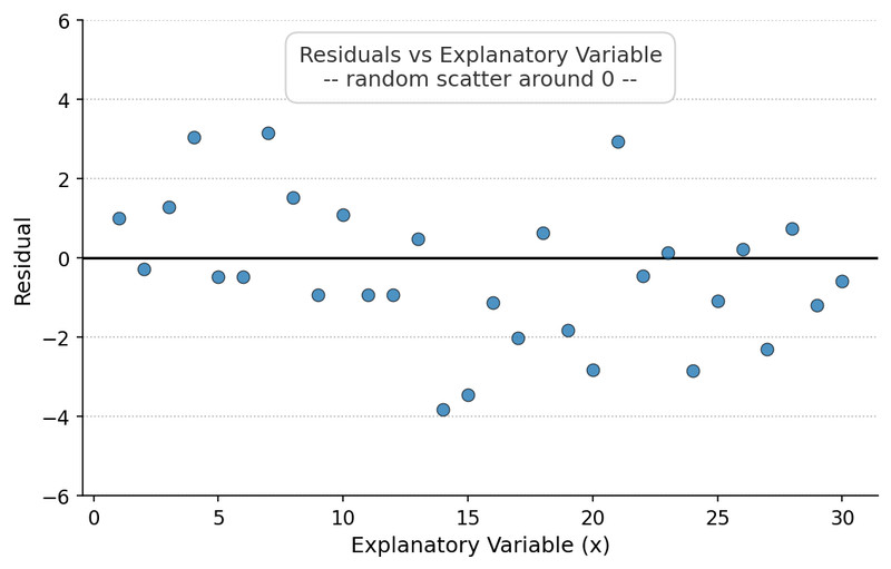
Residual plot with random scatter around 0

The horizontal line at 0 represents perfect predictions. Points above the line are positive residuals. Points below the line are negative residuals.

Residual plots are used to judge whether a linear model is appropriate.

4. How to Interpret a Residual Plot

What you want to see

• Residuals scattered randomly above and below 0
• Roughly constant spread
• No clear pattern

That “random mess” is actually good. It suggests the linear model captures the relationship.

You’d say:

The residual plot shows no apparent pattern, suggesting a linear model is appropriate.

Patterns that signal problems

Compare the two residual plots below. One supports a linear model. The other clearly does not.

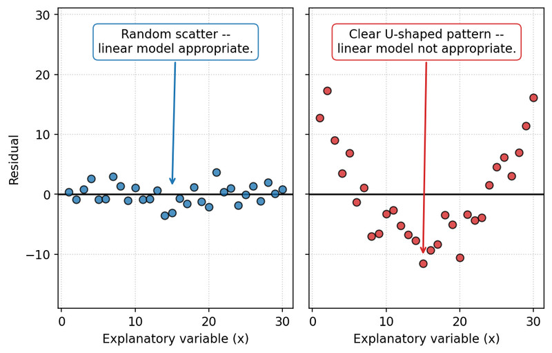
Residual plots: random scatter vs. curved pattern

1. Curved pattern (U-shape or upside-down U)
   The relationship is not linear. A line is missing curvature.
2. Fan shape (increasing or decreasing spread)
   The variability changes as x increases. Not constant variance.
3. Clusters or structure
   Suggests different groups or missing variables.

If there’s a visible pattern, the model is missing something systematic.

5. Using Residual Plots to Evaluate Models

Residual plots answer one main question:

Is a linear model appropriate?

• Random scatter → linear form is supported.
• Clear pattern → linear model is not appropriate.

The residual plot does not tell you:

• Strength of association (that’s r and the scatterplot)
• Causation
• Whether predictions are “good enough” overall

It strictly checks form.

On free-response questions, students often lose points by saying “the model is good” instead of referencing the pattern (or lack of pattern) in the residual plot. Always tie your conclusion to what you see.