Topic 4.3 Notes – Introduction to Probability

1. Probability as Long-Run Relative Frequency

In AP Stats, probability is about long-run behavior, not a single trial.

If you repeat a random process many, many times, the relative frequency of an event (how often it happens ÷ total trials) will get closer and closer to the true probability.

Here’s what that looks like with repeated coin flips:

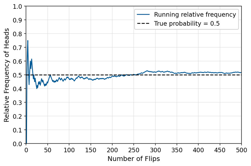
Running relative frequency of heads over 500 flips

Early on, the proportion jumps around a lot. After just a few flips, one extra head or tail makes a big difference. As the number of trials grows, the running proportion settles in near 0.5, the true probability shown by the horizontal line.

If an event has probability 0.30, that does not mean it will happen 3 out of the next 10 times. It means that in a very large number of repetitions, about 30% of outcomes are expected to be that event.

When you interpret probability on a test, use language like:

• “In the long run, about 30% of randomly selected students are expected to…”
• “The probability that a randomly selected voter supports the measure is 0.42.”

Avoid words like “guaranteed” or “will happen.” Probability describes likelihood, not certainty (unless it’s 1).

2. Sample Space and Events

Before calculating probability, you need a clear picture of the random process.

Sample Space

The sample space (S) is the set of all possible outcomes.

Two requirements:

• Outcomes must be clearly defined.
• Outcomes must not overlap at this level.

Examples:

• Randomly select a day of the week
  $S = \{\text{Mon, Tue, Wed, Thu, Fri, Sat, Sun}\}$
• Spin a spinner labeled 1, 2, 3
  $S = \{1, 2, 3\}$

If you leave something out, your probabilities will be wrong because they won’t add to 1.

Events

An event is any subset of the sample space.

• One outcome: “Select Wednesday.”
• Multiple outcomes: “Select a weekend day” → {Sat, Sun}

If event A is “weekend day,” then $P(A)$ measures how much of the sample space belongs to that event.

Big idea: probability measures the proportion of the sample space that makes the event happen.

3. The Basic Probability Rules

These four rules show up constantly. You should see how they fit together.

a. Equally Likely Outcomes Rule

If all outcomes are equally likely,

$$P(A) = \frac{\text{number of outcomes in event A}}{\text{total number of outcomes in } S}$$

Example: Roll a fair six-sided die.
Event A = “roll a multiple of 3” → {3, 6}

$$P(A) = \frac{2}{6} = \frac{1}{3}$$

Only use this rule when the problem clearly implies equal likelihood (fair die, random selection, well-shuffled deck). The AP sometimes hides unequal probabilities in wording.

b. Probability Is Between 0 and 1

$$0 \le P(A) \le 1$$

• 0 → impossible
• 1 → certain

If you calculate −0.2 or 1.4, something went wrong. This is your built-in error check.

c. Total Probability Is 1

The probabilities of all outcomes in the sample space must add to 1.

If a model says:

• P(A) = 0.4
• P(B) = 0.35
• P(C) = 0.30

That sums to 1.05. Invalid model.

On multiple choice, this is sometimes the fastest way to eliminate answers.

d. The Complement Rule

The complement of event A, written $A^c$ or A′, means “not A.”

$$P(A^c) = 1 - P(A)$$

This rule is powerful for phrases like:

• “At least one”
• “Not defective”
• “Does not pass”

Example: If 12% of packages are damaged,

$$P(\text{not damaged}) = 1 - 0.12 = 0.88$$

Often it’s much easier to compute the complement and subtract from 1 than to count everything directly.

4. Applying Probability on Assessments

When solving a problem, your thinking should flow like this:

1. Describe the random process.
2. List or describe the sample space.
3. Identify the event.
4. Decide whether outcomes are equally likely.
5. Apply the correct rule.
6. Check that your answer is between 0 and 1.

When writing a conclusion in context, be specific:

“The probability that a randomly selected laptop from this shipment is defective is 0.08. In the long run, about 8% of laptops from this shipment are expected to be defective.”

Name the population. Name the event. Use long-run language.

Common mistakes I see every year:

• Assuming equal likelihood without justification.
• Forgetting to include all outcomes.
• Not using the complement for “at least” questions.
• Giving a numerical answer with no context sentence on FRQs.