Topic 1.6 Notes – Describing the Distribution of a Quantitative Variable
1. What It Means to Describe a Distribution
When you describe a distribution, you are summarizing the overall pattern of the data in one variable.
You are answering:
- What does it look like?
- Where is it centered?
- How spread out is it?
- Is anything unusual?
This is descriptive statistics. You are not making claims about a larger population. You’re just describing the graph or dataset in front of you.
A complete description almost always includes:
- Shape
- Center
- Spread (variability)
- Unusual features (outliers, gaps, clusters, multiple peaks)
If one of those is missing on a quiz or FRQ, you’re usually losing points.
2. Shape and Unusual Features
Overall Shape
There are three main shapes you need to recognize. The diagrams below show what each one typically looks like.
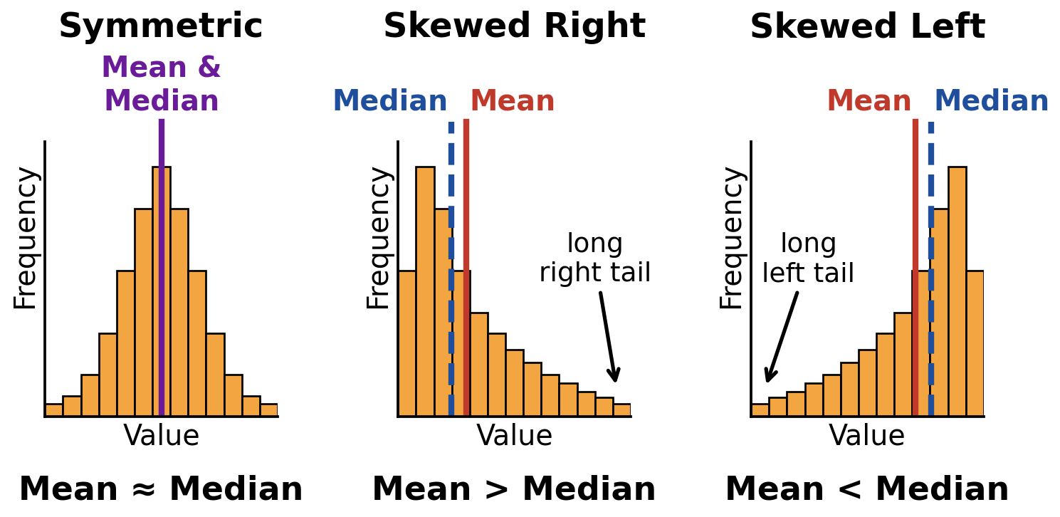
Symmetric, right-skewed, and left-skewed distributions. Each skew is named for its long tail, and the mean is pulled toward that tail.
Symmetric
- Left and right sides are roughly mirror images.
- Tails are about equal length.
- Mean and median are close together.
Skewed Right (Positive Skew)
- Right tail is longer.
- Most values are on the lower end.
- High values pull the mean to the right.
- Mean > median.
Skewed Left (Negative Skew)
- Left tail is longer.
- Most values are on the higher end.
- Low values pull the mean to the left.
- Mean < median.
Always name skewness by the direction of the tail, not where most of the data are. That’s a super common mistake.
Number of Peaks (Modality)
- Unimodal → one clear peak
- Bimodal → two distinct peaks
- Multimodal → more than two peaks
- Uniform → bars about the same height; no obvious peak
Bimodal or multimodal distributions often suggest multiple groups in the data. For example, mixing freshmen and seniors’ heights in one graph could create two peaks.
Unusual Features
Outliers
- Values unusually small or large compared to the rest.
- Often visually isolated.
- Can strongly affect the mean and standard deviation.
An outlier isn’t automatically wrong. Just note it.
Gaps
- Areas with no data values.
- Often separate clusters.
Clusters
- Groups of values packed together.
- Usually separated by gaps.
If you see clusters or gaps, mention them. That often earns the “unusual features” point on FRQs.
3. Center of a Distribution
The center is a typical value.
Mean
- Arithmetic average.
- Uses every data value.
- Sensitive to outliers.
- Best for symmetric distributions.
Median
- Middle value when ordered.
- Resistant to outliers.
- Best for skewed distributions.
Mode
- Most frequent value.
- Mostly used to describe modality, not center, in AP Stats.
Key relationships:
- Right-skewed → mean > median
- Left-skewed → mean < median
- Symmetric → mean ≈ median
Choosing center:
| Shape | Best Measure of Center |
|---|---|
| Symmetric | Mean |
| Skewed or with outliers | Median |
4. Spread of a Distribution
Spread describes variability - how far values are from the center.
Range
- Uses only two values.
- Very sensitive to outliers.
Interquartile Range (IQR)
- Spread of the middle 50%.
- Resistant to outliers.
- Paired with the median.
Standard Deviation (s)
- Measures typical distance from the mean.
- Uses all data values.
- Sensitive to outliers.
- Paired with the mean.
Choosing spread:
| Shape | Best Measure of Spread |
|---|---|
| Symmetric | Standard deviation |
| Skewed or with outliers | IQR |
Always pair:
- Mean with standard deviation
- Median with IQR
Mixing them is a red flag on the AP exam.
5. Writing a Complete Description
A strong description usually sounds like this:
“The distribution of daily screen time for these students is right-skewed and unimodal. It is centered at about 3 hours. The IQR is about 1.5 hours, indicating moderate variability. There is a high outlier around 9 hours.”
Notice:
- Shape first
- Then center (with units)
- Then spread (with units)
- Then unusual features
- All in context
Avoid saying “normal” unless you justify it by describing symmetry and shape.
Key Takeaways
Describing a Quantitative Distribution
Describe it by shape, center, spread, and unusual features like outliers, gaps, or clusters.
Symmetric Distribution
The left and right sides are approximately mirror images around the center.
Skewed Right / Positive Skew and Skewed Left / Negative Skew
Right-skewed has a longer right tail; left-skewed has a longer left tail.
Modes, Unimodal, Bimodal, and Approximately Uniform
One peak is unimodal, two prominent peaks are bimodal, and similar bar heights are approximately uniform.
Outlier
A value unusually small or large compared with the rest of the data.
Gap
A region between data values where no observations occur.
Cluster
A concentration of data values, often separated from others by gaps.
Mean, Median, and Mode as Measures of Center
Mean is the average, median is the middle ordered value, and mode is the most frequent value.
Range, Standard Deviation, and Interquartile Range as Measures of Spread
Range is max minus min, standard deviation measures typical distance from the mean, and IQR is Q3 minus Q1.
Mean and Standard Deviation vs. Median and IQR
Use mean with standard deviation for roughly symmetric data; use median with IQR for skewed data or outliers.
Descriptive Statistics
Numerical and graphical summaries that describe observed data without generalizing to a population.
Notes
Describing a Quantitative Distribution
Describe it by shape, center, spread, and unusual features like outliers, gaps, or clusters.
Symmetric Distribution
The left and right sides are approximately mirror images around the center.
Skewed Right / Positive Skew and Skewed Left / Negative Skew
Right-skewed has a longer right tail; left-skewed has a longer left tail.
Modes, Unimodal, Bimodal, and Approximately Uniform
One peak is unimodal, two prominent peaks are bimodal, and similar bar heights are approximately uniform.
Outlier
A value unusually small or large compared with the rest of the data.
Gap
A region between data values where no observations occur.
Cluster
A concentration of data values, often separated from others by gaps.
Mean, Median, and Mode as Measures of Center
Mean is the average, median is the middle ordered value, and mode is the most frequent value.
Range, Standard Deviation, and Interquartile Range as Measures of Spread
Range is max minus min, standard deviation measures typical distance from the mean, and IQR is Q3 minus Q1.
Mean and Standard Deviation vs. Median and IQR
Use mean with standard deviation for roughly symmetric data; use median with IQR for skewed data or outliers.
Descriptive Statistics
Numerical and graphical summaries that describe observed data without generalizing to a population.
