Topic 7.4 Notes – Setting Up a Test for a Population Mean

What a One-Sample t-Test Is

A one-sample t-test is used to test a claim about a population mean $\mu$ when the population standard deviation $\sigma$ is unknown. That’s almost always the case in real data, so we use the t-distribution.

You’re in one-sample t-test territory when:

• The variable is quantitative (heights, times, scores, weights, etc.)
• You have one sample
• You are comparing the sample mean $\bar{x}$ to a claimed value

The idea: if the claim about $\mu$ were true, how likely would it be to get a sample mean as far from that value as we did?

Matched Pairs = One Sample of Differences

Matched pairs often look like two samples, but they aren’t.

Examples:

• Before/after measurements
• Same person under two conditions
• Twins matched on characteristics

Treat this as:

1. Compute a difference for each pair.
2. Let $\mu_d$ = true mean difference.
3. Run a one-sample t-test on the differences.

⚠️ Define the subtraction clearly (e.g., after − before). If you switch the order, the sign changes and so does the direction of your alternative hypothesis.

When to Use It (and When Not To)

You’ll usually see wording like:

• “Is there convincing evidence…”
• “Do the data suggest…”

Those phrases signal a significance test.

If:

• Data are quantitative
• You’re testing a claim about a mean
• $\sigma$ is unknown

→ Use a one-sample t-test.

If the data are categorical (like proportions), this is the wrong procedure. That’s a different test.

Hypotheses for a Population Mean

Always define your parameter in context.

Regular One-Sample t-Test

Let $\mu$ = true mean ___ (in context).

$$H_0: \mu = \mu_0$$

Alternative depends on the question:

• $H_a: \mu \ne \mu_0$ (two-sided)
• $H_a: \mu > \mu_0$ (right-tailed)
• $H_a: \mu < \mu_0$ (left-tailed)

Key reminders:

• The null always has equality.
• The alternative comes from the wording, not your sample result.
• Never write hypotheses using $\bar{x}$. Use $\mu$.

Matched Pairs Hypotheses

Let $\mu_d$ = true mean difference (state subtraction order).

$$H_0: \mu_d = 0$$

$$H_a: \mu_d \ne 0 \quad \text{or} \quad \mu_d > 0 \quad \text{or} \quad \mu_d < 0$$

The value 0 represents “no difference.”

On free-response questions, students often lose points by forgetting to define $\mu$ or $\mu_d$ in context. Write it out clearly.

Conditions for Inference

Before calculating anything, check Random, Independent, Normal (RIN).

1. Random

Data come from:

• A random sample, or
• A randomized experiment

Say this using the wording from the problem.

2. Independent

If sampling without replacement, check the 10% condition:

$$\frac{n}{N} \le 0.10$$

In context, you might say:

It is reasonable to believe there are at least 10n students in the population.

3. Normal (Shape)

We need the sampling distribution of $\bar{x}$ to be approximately normal.

You can justify this if:

• $n \ge 30$ (Central Limit Theorem), or
• Population is stated to be approximately normal, or
• If $n < 30$, the sample data show no strong skewness or outliers.

For matched pairs, check normality of the differences, not the original variables.

Strong skewness means the distribution has a long tail to the right or left, like the skewed-left and skewed-right histograms below.

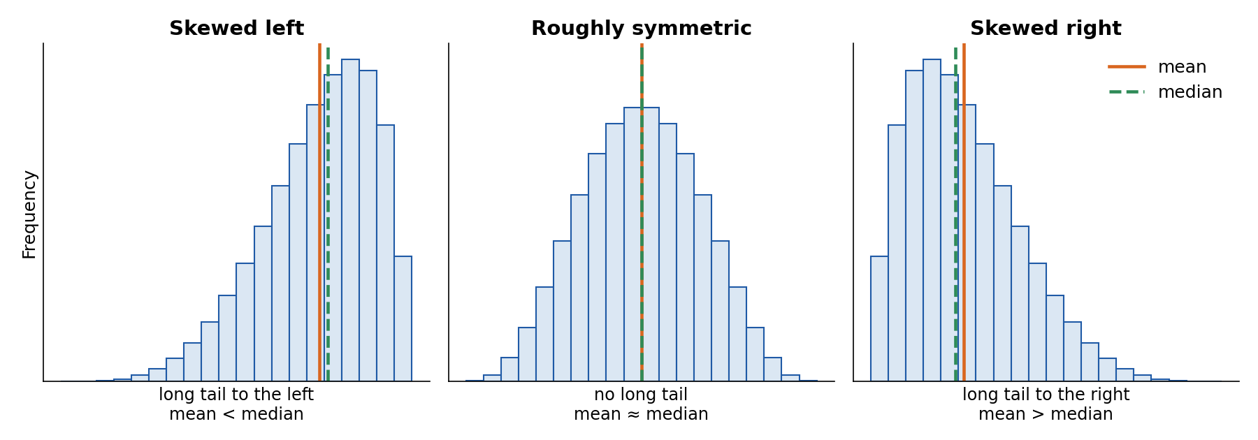
Skewed left, roughly symmetric and skewed right, with the mean and median marked

If your sample is small and looks like one of the skewed shapes, the t-procedure is questionable.

Test Statistic and Significance Level

The test statistic measures how many standard errors the sample mean is from the hypothesized mean.

$$t = \frac{\bar{x} - \mu_0}{s / \sqrt{n}}$$

Degrees of freedom: $$df = n - 1$$

For matched pairs, replace $\bar{x}$ with $\bar{d}$ and $s$ with $s_d$.

Significance Level $\alpha$

• $\alpha$ = probability of a Type I error
• Commonly 0.05
• Reject $H_0$ if p-value < $\alpha$

In a two-sided test with $\alpha = 0.05$, the 0.05 is split evenly between the two tails of the t-distribution.

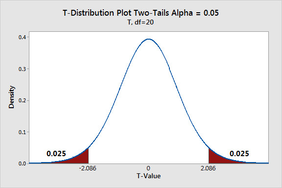
Two-tailed t-distribution with $\alpha = 0.05$ (df = 20)

Each tail has area 0.025. Values beyond the critical t-scores fall in the rejection region.

Connection to confidence intervals:

A two-sided test at $\alpha = 0.05$ matches a 95% confidence interval.

If $\mu_0$ is outside the interval → reject $H_0$.