Topic 9.2 Notes – Confidence Intervals for the Slope of a Regression Model

1. What the slope of a regression model represents

In the population, the true linear relationship is written as

$$\mu_y = \alpha + \beta x$$

• $\mu_y$ is the mean response at a given value of $x$.
• $\beta$ is the population slope.

Interpretation of $\beta$:
For each 1-unit increase in $x$, the mean value of $y$ changes by $\beta$ units.

From a sample, we compute the least-squares line:

$$\hat{y} = a + bx$$

• $b$ is the sample slope.
• $b$ is a point estimate of $\beta$.

How variability enters

Not every point falls exactly on the line. The difference between an observed value and its predicted value is a residual:

$$\text{residual} = y_i - \hat{y}_i$$

These residuals estimate how far actual responses vary from the true population line.

The standard deviation of the residuals estimates the true variability around the regression line:

$$s = \sqrt{\frac{\sum (y_i - \hat{y}_i)^2}{n - 2}}$$

We divide by $n - 2$ because we estimated two parameters, $\alpha$ and $\beta$.

Important sampling facts:

• The sampling distribution of $b$ has mean $\mu_b = \beta$.
• Its standard deviation depends on:
  • residual variability (how scattered points are vertically),
  • spread of the $x$-values,
  • sample size.

Because we don’t know the population standard deviation $\sigma$, we use a t‑interval for the slope.

2. Conditions for a confidence interval for the slope

All four must be checked and stated in context.

Linear

The relationship between $x$ and $y$ is linear.
Check the residual plot. You want random scatter around 0.

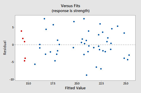
Residual plot showing random scatter around 0

Equal spread

The variability of $y$ is roughly constant for all $x$.
On the same residual plot, look for no funnel or fan shape as fitted values increase.

Independence

• Data come from a random sample or randomized experiment.
• If sampling without replacement, verify $n \le 0.10N$.

Normal

For each value of $x$, the distribution of $y$ is approximately normal.
Check a histogram or normal probability plot of residuals.

If residuals are skewed, you need $n \ge 30$ for the t‑procedure to be reliable.

3. Constructing the confidence interval for the slope

This is a t-interval for $\beta$.

Formula

$$b \pm t^* (SE_b)$$

Where:

• Point estimate: $b$
• Degrees of freedom: $\text{df} = n - 2$
• Margin of error: $t^* \times SE_b$

The standard error of the slope is

$$SE_b = \frac{s}{s_x \sqrt{n - 1}}$$

• $s$ = standard deviation of residuals
• $s_x$ = sample standard deviation of the $x$-values

What affects the margin of error?

The margin of error equals $t^* \cdot SE_b$.

It gets larger when:

• confidence level increases (bigger $t^*$),
• residual variability $s$ is large,
• spread in $x$ (small $s_x$) is small,
• sample size is small.

It shrinks with:

• larger $n$,
• less vertical scatter,
• wider spread of $x$-values.

On your calculator, LinRegTInt will compute this directly using your data lists.

4. Interpreting the interval correctly

A complete interpretation always includes:

• confidence level,
• the population parameter $\beta$,
• the variables in context,
• “mean” language.

Example structure:

“We are 95% confident that the true slope $\beta$ describing the relationship between [explanatory variable] and the mean [response variable] is between ___ and ___.”

Then explain meaning:

“For each 1-unit increase in [x], the mean [y] changes by between ___ and ___ units.”

What the confidence level means:

If we repeated this sampling process many times, about $C\%$ of the intervals would capture the true $\beta$.
The parameter is fixed. The interval changes from sample to sample.

5. Common mistakes

• Using $z$ instead of $t$.
• Using df = $n - 1$ instead of $n - 2$.
• Interpreting the interval as predicting individual $y$-values.
• Saying there is a $C\%$ probability that $\beta$ is in this interval.
• Forgetting to check residual plots before computing.

Remember, this interval estimates the population slope, not the intercept and not individual outcomes.