Topic 5.3 Notes – The Central Limit Theorem

What a Sampling Distribution Is

A sampling distribution of a statistic is the distribution of that statistic’s values for all possible samples of size $n$ from a population.

Key idea: we are not talking about raw data values. We are talking about a statistic like $\bar{x}$.

If you:

• Take a random sample of size $n$,
• Compute $\bar{x}$,
• Repeat this over and over,

the collection of those $\bar{x}$ values forms the sampling distribution of $\bar{x}$.

For the sample mean:

$$\mu_{\bar{x}} = \mu$$

$$\sigma_{\bar{x}} = \frac{\sigma}{\sqrt{n}}$$

So:

• The mean of the sampling distribution equals the population mean. That makes $\bar{x}$ an unbiased estimator.
• The spread shrinks as $n$ increases because of the $\sqrt{n}$ in the denominator.

That shrinking spread is why larger samples give more consistent averages.

The Central Limit Theorem

The Central Limit Theorem (CLT) says:

When the sample size is sufficiently large, the sampling distribution of the sample mean is approximately normal, regardless of the population’s shape.

So even if the population is skewed or messy, the distribution of sample means becomes bell-shaped when $n$ is large enough.

Here’s the visual idea. Start with a right-skewed population, then look at what happens to the distribution of $\bar{x}$ as $n$ increases:

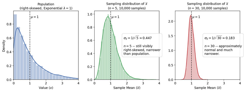
Population vs. sampling distributions as n increases

Notice in the picture:

• The original population is clearly right-skewed.
• For $n = 5$, the sampling distribution is still a bit skewed, but more concentrated.
• For $n = 30$, the sampling distribution is approximately normal and much narrower.

As sample size increases:

• Shape becomes more normal.
• Spread decreases.
• Center stays at $\mu$.

Conditions for Using the CLT

You must check:

1. Random
   The data come from a random sample or randomized experiment.

2. Independent
   Use the 10% condition when sampling without replacement:
   $n \le 0.1N$

3. Large enough sample size

   • Rule of thumb: $n \ge 30$
   • If the population is already normal, any $n$ works.
   • If the population is heavily skewed, you may need more than 30.

On a free response question, you need to literally say that the sampling distribution is approximately normal by the Central Limit Theorem. If you skip naming it, you can lose credit.

Using the CLT for Probabilities About a Mean

You use the CLT when a question asks about:

• An average
• A mean
• A symbol like $\bar{x}$

You are not finding probabilities for individual observations. You are finding probabilities for sample means.

The standardized value is:

$$z = \frac{\bar{x} - \mu}{\sigma/\sqrt{n}}$$

Notice the denominator. Students constantly use $\sigma$ instead of $\sigma/\sqrt{n}$. That mistake changes everything.

Once you find $z$, use the normal distribution to get the probability.

If you are writing a conclusion on an FRQ, include context. For example, say “the probability that the mean wait time for samples of 40 customers exceeds 6 minutes is…” not just “the probability is 0.12.”

Simulating Sampling Distributions

Instead of formulas, you can build a sampling distribution using simulation.

To simulate a sampling distribution:

1. Generate a random sample of size $n$ from a population.
2. Compute the statistic (like $\bar{x}$).
3. Repeat many times.
4. Graph the results.

If you simulate this process hundreds or thousands of times and record each sample mean, you get a distribution like the one below.

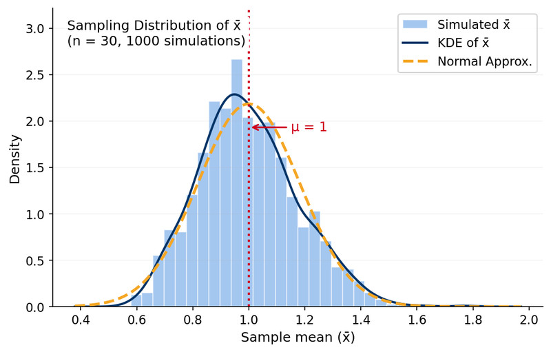
Simulated sampling distribution of $\bar{x}$ (n = 30, 1000 samples)

Each bar represents many simulated sample means. Notice how the distribution is centered near the population mean and has a roughly normal shape.

As the number of simulated samples increases, the histogram better approximates the true sampling distribution.

This is often done with technology in class to see the CLT in action.

Randomization Distributions

A randomization distribution is different.

Instead of sampling from a population, you:

• Assume a null value for a parameter.
• Reassign or shuffle data repeatedly.
• Calculate the statistic each time.

In a randomized experiment, that means:

• Keep the response values fixed.
• Randomly reassign them to treatment groups many times.
• Compute the difference in means (or other statistic) each time.

This models what would happen by chance alone under the null hypothesis.

So remember:

• Sampling distribution → variability of a statistic across random samples.
• Randomization distribution → variability of a statistic under a null assumption, built by simulation.