Topic 5.7 Notes – Sampling Distributions for Sample Means

1. What the Sampling Distribution of x̄ Is

Picture taking a random sample of size $n$, calculating its mean, then repeating that process over and over. Each time you get a different $\bar{x}$.

The sampling distribution of $\bar{x}$ is the distribution of all those possible sample means.

Important grounding:

• Population → parameters:
  • Mean $\mu$
  • Standard deviation $\sigma$
• Sample → statistics:
  • Mean $\bar{x}$
  • Standard deviation $s$

This topic is about how $\bar{x}$ behaves across many samples, not about individual data values.

We care because it lets us:

• Predict how close $\bar{x}$ is likely to be to $\mu$
• Calculate probabilities about sample means
• Build confidence intervals and hypothesis tests later

Here’s the idea visually. The top row shows different population distributions. The rows underneath show the sampling distributions of $\bar{x}$ when $n = 5$ and when $n = 30$.

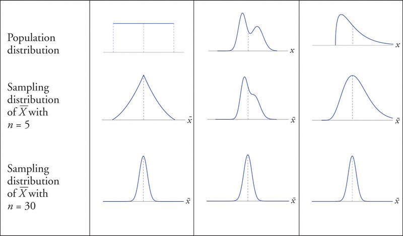
Population distributions and sampling distributions of $\bar{x}$ for $n = 5$ and $n = 30$

Notice how the sampling distribution is typically less spread out than the population, and how it becomes more nearly normal and tighter as the sample size increases.

2. Mean and Standard Deviation of x̄

Assume we are randomly sampling with replacement from a population with mean $\mu$ and standard deviation $\sigma$.

Center of the sampling distribution

$$\mu_{\bar{x}} = \mu$$

The mean of all possible sample means equals the population mean.

That makes $\bar{x}$ an unbiased estimator of $\mu$. On average, sample means hit the true mean.

If a problem gives you $\mu = 72$, then the center of the sampling distribution is automatically 72. No extra work.

Spread of the sampling distribution

$$\sigma_{\bar{x}} = \frac{\sigma}{\sqrt{n}}$$

This is the standard error (SE) of the mean.

What affects it?

• Larger $\sigma$ → more variability in $\bar{x}$
• Larger $n$ → divide by bigger $\sqrt{n}$ → smaller variability

So bigger samples give more precise estimates.

Quick example:
If $\sigma = 12$ and $n = 36$,

$$\sigma_{\bar{x}} = \frac{12}{\sqrt{36}} = \frac{12}{6} = 2$$

Even though individuals vary by 12 units, sample means only vary by 2.

Common mistake on tests: using $\sigma$ instead of $\sigma / \sqrt{n}$ when calculating a z-score for a sample mean.

Sampling without replacement and the 10% condition

The formula $\sigma / \sqrt{n}$ is exact for sampling with replacement.

If sampling without replacement, the true standard deviation is slightly smaller.

On the AP exam:

• If $n \le 0.10N$, the difference is negligible.
• This is the 10% condition and it supports independence.

If the 10% condition is met, just use $\sigma / \sqrt{n}$ like normal.

3. When the Sampling Distribution Is Normal

To use normal probability calculations, the sampling distribution must be (approximately) normal.

Two situations:

Population is normal

If the population distribution is normal, then the sampling distribution of $\bar{x}$ is exactly normal for any sample size.

Even if $n = 5$, you’re good.

Population is not normal

If the population is not normal, we use the Central Limit Theorem (CLT).

The CLT says:

As $n$ gets large, the distribution of $\bar{x}$ becomes approximately normal, regardless of population shape.

Rule of thumb:

• $n \ge 30$ → usually large enough.

If the population is extremely skewed or has strong outliers, you may need a larger $n$.

On free-response, you must justify normality by stating either:

• Population is normal
• $n \ge 30$, so CLT applies

4. Using the Sampling Distribution to Find Probabilities

When finding a probability involving a sample mean:

1. Check normal condition (population normal or $n \ge 30$).
2. Identify
   • $\mu_{\bar{x}} = \mu$
   • $\sigma_{\bar{x}} = \frac{\sigma}{\sqrt{n}}$
3. Compute
   $$z = \frac{\bar{x} - \mu}{\sigma / \sqrt{n}}$$
4. Use normalcdf or a z-table.

Example setup:

Suppose $\mu = 50$, $\sigma = 8$, $n = 64$.

Then
$$\sigma_{\bar{x}} = \frac{8}{\sqrt{64}} = 1$$

If asked for $P(\bar{x} > 52)$,

$$z = \frac{52 - 50}{1} = 2$$

Then find $P(Z > 2)$.

Be careful with interpretation. You are talking about sample means of size 64, not individual values.

Correct style:
“There is a ___% chance that the mean of a random sample of 64 observations will exceed 52.”

5. Interpreting in Context

Always:

• Mention sample means
• Include correct units
• Reference the population

Remember:

• $\mu$ is fixed.
• $\bar{x}$ varies from sample to sample.

This variability is exactly what the sampling distribution models.