Topic 5.2 Notes – The Normal Distribution, Revisited

1. The Normal Distribution

A normal distribution is a continuous probability distribution with a very specific shape:

• Bell-shaped
• Symmetric
• Unimodal (one peak)
• Centered at the mean $\mu$

For a normal distribution:

• Mean = median = mode
• Total area under the curve = 1 (100%)
• 50% of the area is on each side of $\mu$

Continuous random variable reminder

A continuous random variable can take any value in an interval.
Example: If you glance at a clock at a random time, the probability the minute hand is between the 3 and 6 is $\frac{1}{4}$. That’s an interval.

For continuous variables:
$$P(X = a) = 0$$

Probabilities are assigned to intervals, not single values.

Area = Probability

In a normal distribution, area under the curve over an interval = probability that $X$ falls in that interval.

If weights of apples are normally distributed, the area between 140 g and 160 g represents the probability a randomly chosen apple weighs in that range.

Describing a normal distribution

Always describe using:

• Center → $\mu$
• Spread → $\sigma$
• Shape → symmetric, bell-shaped

Empirical Rule

For quick mental estimates:

• 68% within $1\sigma$
• 95% within $2\sigma$
• 99.7% within $3\sigma$

The diagram below shows how those percentages are distributed symmetrically around the mean.

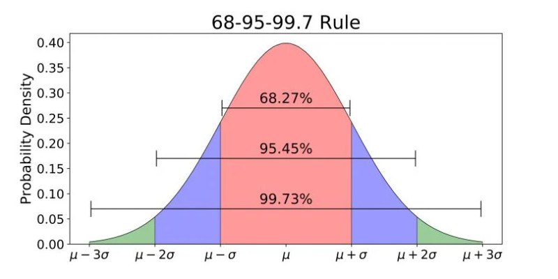
Empirical Rule for a normal distribution

That 95% within 2σ shows up constantly in inference later.

2. Z-Scores and the Standard Normal Model

A z-score tells how many standard deviations a value is from the mean.

$$z = \frac{x - \mu}{\sigma}$$

• Positive $z$ → above the mean
• Negative $z$ → below the mean
• Larger magnitude → farther from the mean

Why we standardize

Standardizing converts any normal distribution into the standard normal distribution:

• Mean = 0
• SD = 1

Then you can use:

• Z-table
• normalcdf
• invNorm

Calculating probabilities step by step

Suppose exam scores are normal with $\mu = 82$, $\sigma = 6$. Find $P(X \le 90)$.

1. Sketch and shade left of 90.
2. Standardize:
   $$z = \frac{90 - 82}{6} = \frac{8}{6} = 1.33$$
3. Use normalcdf(-1E99, 90, 82, 6)
   or normalcdf(-1E99, 1.33, 0, 1)

The result is the area to the left, which is the probability a randomly selected student scored 90 or below.

Common calculator forms:

• $P(X \le a)$
• $P(X \ge b)$
• $P(a < X < b)$

Common mistakes I see on quizzes:

• Forgetting to shade first
• Mixing up left vs right tail
• Using invNorm when you need normalcdf

3. Finding Values from a Given Area

Now we reverse it. You’re given an area and must find the boundary value.

You work backward.

General process

1. Sketch and shade the given area.
2. Find the corresponding z-score using table or invNorm.
3. Convert back:
   $$x = \mu + z\sigma$$

Interpreting statements correctly

These phrases matter.

• Lowest p%
  $P(X \le x_a) = \frac{p}{100}$
  Left-tail area.
• Highest p%
  $P(X \ge x_b) = \frac{p}{100}$
  Right-tail area.
• Middle p%
  $P(x_a < X < x_b) = \frac{p}{100}$
  Usually symmetric around the mean.
• Most extreme p%
  Split into two tails:
  $$P(X \le x_a) = \frac{p}{200}, \quad P(X \ge x_b) = \frac{p}{200}$$

If a problem says “most extreme 8%,” that means 4% in each tail. Students miss that all the time.

Remember: invNorm expects left-tail area, so adjust accordingly.

4. When Is a Normal Model Appropriate?

Normal distributions are:

• Symmetric
• Bell-shaped
• No strong skew
• No extreme outliers

If the distribution is heavily skewed, the normal model won’t approximate probabilities well.

For sampling distributions (quick review):

• Proportions → Large Counts condition
  $np \ge 10$ and $n(1 - p) \ge 10$
• Means → $n \ge 30$ or population is normal

If asked whether a normal model is appropriate, say something like:

“The histogram of battery lifetimes appears approximately symmetric and bell-shaped with no outliers, so using a normal model to approximate probabilities is reasonable.”

Always reference shape.