Topic 7.2 Notes – Constructing a Confidence Interval for a Population Mean

1. What the t-Distribution Is and Why We Use It

When estimating a population mean $\mu$, we rarely know the population standard deviation $\sigma$. So we replace it with the sample standard deviation $s$.

That substitution adds extra variability. Because of that, the standardized statistic

$$t = \frac{\bar{x} - \mu}{s/\sqrt{n}}$$

follows a t-distribution, not a normal distribution.

How the t-distribution compares to normal

In the graph below, both curves are centered at 0. The green t-curve with df = 1 has a lower peak and thicker tails than the blue normal curve.

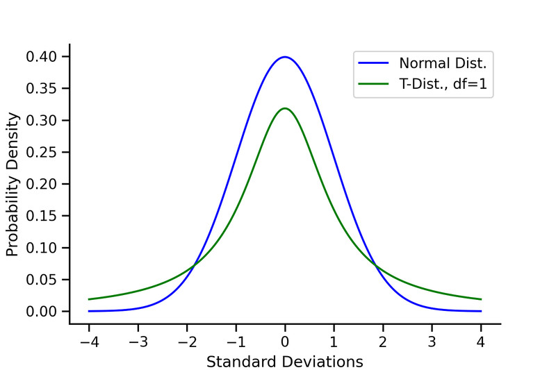
Normal distribution vs. t-distribution (df = 1)

Key properties:

• Symmetric, bell-shaped, centered at 0
• Heavier tails than the normal distribution
  • More area in the extremes
  • Accounts for uncertainty from using $s$ instead of $\sigma$

Degrees of freedom (df)

For a one-sample mean:

$$\text{df} = n - 1$$

As df increases:

• Tails get thinner
• The t-curve gets closer to the normal curve

Large sample → t ≈ normal
Small sample → noticeably wider tails → larger critical values

That’s why small samples produce wider intervals.

2. When to Use a One-Sample t-Interval

You use a one-sample t-interval when:

• You’re estimating a population mean $\mu$
• Data come from one quantitative variable
• $\sigma$ is unknown (which is typical)
• Data come from:
  • A random sample, or
  • A randomized experiment (if estimating a mean response)

If the problem says “average,” “mean,” or “how much on average,” your brain should immediately think: mean → probably t.

Matched Pairs

Sometimes data come in pairs, like:

• Before/after measurements
• Twin studies
• Matched subjects

Treat this as one sample of differences:

1. Compute each pair’s difference.
2. Use those differences as your sample.
3. Construct a one-sample t-interval for the mean difference $\mu_d$.

You are not doing two-sample inference here. Once differences are calculated, it’s a one-sample problem.

3. Conditions for a One-Sample t-Interval

You must check independence and approximately normal sampling distribution.

Random

• Data from a random sample or random assignment
• On written responses, state where randomness came from in context.

Independence

• Observations must be independent.
• If sampling without replacement, check the 10% condition:

$$\frac{n}{N} \leq 0.10$$

In words: it’s reasonable to believe the population is at least 10 times the sample size.

Say it in context, like:
“It is reasonable to believe there are at least 10n students at the school.”

Nearly Normal (Shape)

We need the sampling distribution of $\bar{x}$ to be approximately normal.

• If n ≥ 30 → OK (Central Limit Theorem)
• If n < 30:
  • No strong skewness
  • No outliers

Small sample + strong skew or outliers → do not use t procedures.

4. Constructing the Confidence Interval

All confidence intervals follow:

$$\textbf{Point Estimate} \pm \textbf{Margin of Error}$$

Point Estimate

For a mean:

$$\bar{x}$$

Standard Error

$$\text{SE} = \frac{s}{\sqrt{n}}$$

This measures how much $\bar{x}$ would vary from sample to sample.

Critical Value

• $t^*$ with df = $n - 1$
• Found using a t-table or calculator (invT or TInterval)

Higher confidence level → larger $t^*$

Margin of Error

$$\text{ME} = t^* \left(\frac{s}{\sqrt{n}}\right)$$

Full Formula

$$\bar{x} \pm t^*\left(\frac{s}{\sqrt{n}}\right)$$

You don’t need to memorize this. Build it from statistic ± (critical value × SE).

5. Interpreting the Confidence Interval

Correct wording matters.

Proper interpretation:

“I am 95% confident that the true population mean of [context] is between [lower] and [upper].”

Must include:

• Confidence level
• Context
• Clear reference to the true population mean

What 95% confident means:

If we took many random samples and built intervals this way, about 95% of those intervals would capture the true $\mu$.

The parameter is fixed. The interval changes.

Never say:
“There is a 95% probability that $\mu$ is in this interval.”

What Makes an Interval Wider?

Since

$$\text{ME} = t^* \cdot \frac{s}{\sqrt{n}}$$

Wider interval if:

• Higher confidence level
• Larger variability $s$
• Smaller sample size

Larger $n$ shrinks the interval because it reduces the standard error.