Topic 4.6 Notes – Approximating Values of a Function Using Local Linearity and Linearization

What local linearity means

If a function $f$ is differentiable at $x = a$, then near that point the graph looks almost straight. The closer you zoom in, the more it resembles a line.

That line is the tangent line at $x = a$.

• The point of tangency is $(a, f(a))$.
• The slope of the tangent line is $f'(a)$.
• Very close to $a$, the function value $f(x)$ is approximately equal to the value of the tangent line.

This idea is called local linearity. We are not saying the function is linear everywhere. Only near that one point.

Here’s what that looks like visually. In this example, $f(x)=\ln(x)$ and the tangent line is drawn at $x=1$:

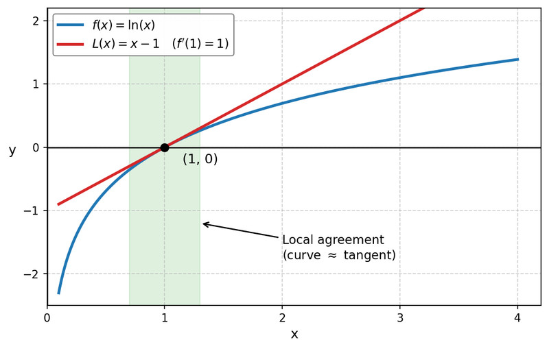
Local linearity: $f(x)=\ln(x)$ and its tangent line at $x=1$

Notice how near $x=1$, the curve and the line are almost indistinguishable. Farther away, they separate. That “zoomed‑in straightness” is the whole reason linearization works.

The linearization formula

The equation of the tangent line at $x = a$ is

$$L(x) = f(a) + f'(a)(x - a)$$

This is just point-slope form:

• point: $(a, f(a))$
• slope: $f'(a)$

So linearization = tangent line. Same object, different name depending on what we’re doing with it.

Using a tangent line to approximate a value

Suppose you want to approximate $f(b)$, where $b$ is close to $a$, and you know $f(a)$ and $f'(a)$.

Here’s the flow:

1. Compute $f(a)$.
2. Compute $f'(a)$.
3. Write $$L(x) = f(a) + f'(a)(x - a).$$
4. Plug in $x = b$.
5. Use $L(b)$ as your approximation for $f(b)$.

Example idea (typical no-calculator question):

Approximate $\sqrt{9.2}$.

Let $f(x) = \sqrt{x}$ and choose $a = 9$ since that’s easy.

• $f(9) = 3$
• $f'(x) = \frac{1}{2\sqrt{x}}$, so $f'(9) = \frac{1}{6}$

Linearization:

$$L(x) = 3 + \frac{1}{6}(x - 9)$$

Plug in $x = 9.2$:

$$L(9.2) = 3 + \frac{1}{6}(0.2) = 3 + \frac{0.2}{6} \approx 3.0333$$

So $$\sqrt{9.2} \approx 3.0333.$$

On a test, they love giving numbers slightly above or below perfect squares, nice trig values, or simple exponentials.

The key is choosing a smart $a$.

Overestimates and underestimates

Now the subtle part. Whether your approximation is too high or too low depends on concavity near the point.

You determine concavity using $f''(a)$.

If $f''(a) > 0$ (concave up)

• The graph bends upward.
• The tangent line lies below the curve near the point.
• Your linear approximation is an underestimate.

If $f''(a) < 0$ (concave down)

• The graph bends downward.
• The tangent line lies above the curve.
• Your linear approximation is an overestimate.

Here’s the geometry. Focus on the left panel for concave up and the right panel for concave down.

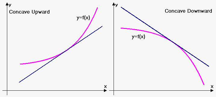
Tangent line position for concave up and concave down

On FRQs, you must justify this using concavity. Saying “it looks like” is not enough. You need a statement like: “Since $f''(a) > 0$, the function is concave up, so the tangent line lies below the curve, making the approximation an underestimate.”

That language earns the point.

What this looks like on AP-style problems

• No-calculator MCQs often test algebra and setup.
• Calculator sections may give a table of values for $f$ and $f'$.
• FRQs frequently combine linearization with a differential equation where you compute $f'(a)$ from the DE first.

The most common mistake is plugging into $f'(x)$ but forgetting to evaluate it at $a$. You need a number for the slope.