Topic 6.2 Notes – Approximating Areas with Riemann Sums

1. What a Riemann Sum Is

A Riemann sum approximates a definite integral by adding areas of simple shapes (usually rectangles or trapezoids) over subintervals of $[a,b]$.

$$\int_a^b f(x)\,dx \approx \sum f(x_i^*)\,\Delta x$$

Break that apart:

• $\Delta x$ = width of each subinterval
• $x_i^*$ = sample point used to find the height
• The sum adds up height × width

Important idea: this gives net signed area.

• Above the x-axis → positive
• Below the x-axis → negative

If you increase the number of subintervals $n$, each $\Delta x$ gets smaller, and the approximation improves.

You might see this when:

• A graph is given
• A table of values is provided
• A formula is given but hard to integrate
• A word problem gives a rate over time

2. The Four Main Approximation Methods

Start by looking at the comparison below. It shows left and right Riemann sums on the same decreasing curve.

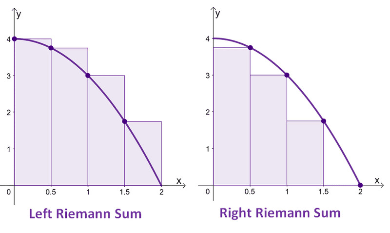
Left vs. right Riemann sums on a decreasing function

Left Riemann Sum $L_n$

Height comes from the left endpoint of each interval.

$$L_n = \sum_{i=1}^{n} f(x_{i-1})\,\Delta x$$

Error depends on whether the function is increasing or decreasing:

• Increasing → underestimate
• Decreasing → overestimate

In the figure above, the function is decreasing, so the left sum overestimates the true area.

Right Riemann Sum $R_n$

Height comes from the right endpoint.

$$R_n = \sum_{i=1}^{n} f(x_i)\,\Delta x$$

• Increasing → overestimate
• Decreasing → underestimate

On that same decreasing graph, the right sum underestimates.

Left/right error is controlled by monotonicity (sign of $f'$).

Midpoint Riemann Sum $M_n$

Height comes from the midpoint of each interval.

$$M_n = \sum f(\text{midpoint})\,\Delta x$$

Now the error depends on concavity, not increasing/decreasing:

• Concave up → underestimate
• Concave down → overestimate

Trapezoidal Sum $T_n$

Instead of rectangles, connect endpoints with straight lines to form trapezoids.

Two equivalent ways to compute:

$$T_n = \frac{L_n + R_n}{2}$$

or for each interval:

$$\text{Area} = \frac{1}{2}(f(x_{i-1}) + f(x_i))\Delta x$$

Concavity controls error:

• Concave up → overestimate
• Concave down → underestimate

Midpoint and trapezoidal behave opposite each other for concavity.

3. How to Compute a Riemann Sum

On a quiz or FRQ, the structure is predictable.

Step 1: Find the width

If partitions are uniform:

$$\Delta x = \frac{b-a}{n}$$

If nonuniform, each interval has its own width. Multiply each height by its own $\Delta x$.

Step 2: Choose sample points

• Left → first value in each interval
• Right → last value
• Midpoint → average of endpoints
• Trapezoidal → use both endpoints

Step 3: Evaluate heights

• Plug into formula
• Read from table
• Estimate from graph

If $\Delta x$ is constant, factor it out. That prevents careless arithmetic mistakes.

On calculator sections, you may compute sums directly. On no-calculator parts, numbers are usually chosen to keep arithmetic manageable.

4. Determining Overestimate or Underestimate

This is tested constantly in conceptual questions.

Increasing or Decreasing (First Derivative Idea)

• $f'(x) > 0$ increasing
  • Left under
  • Right over
• $f'(x) < 0$ decreasing
  • Left over
  • Right under

Concavity (Second Derivative Idea)

• $f''(x) > 0$ concave up
  • Trapezoidal over
  • Midpoint under
• $f''(x) < 0$ concave down
  • Trapezoidal under
  • Midpoint over

Straight-line trapezoids sit above a cup-shaped curve and below a cap-shaped curve.

5. Common AP Traps

• Forgetting integrals are signed area
• Using concavity rules for left/right
• Mixing up endpoints in tables
• Forgetting $\Delta x$
• Ignoring unequal widths in nonuniform partitions