Topic 7.8 Notes – Exponential Models with Differential Equations

The exponential growth and decay differential equation

The core model is

$$\frac{dy}{dt} = ky$$

Here’s what each piece means in context:

• $y(t)$: the quantity changing (population, mass, concentration, position, etc.)
• $\frac{dy}{dt}$: the rate of change of that quantity
• $k$: a constant of proportionality
  • $k > 0$ → growth
  • $k < 0$ → decay
  • Units of $k$ are “per time” (like per year, per hour)

The phrase you’re listening for on a test is:

• “Rate proportional to the amount”
• “Increases at a rate proportional to its size”
• “Decreases at a rate proportional to the amount present”

That wording translates immediately to
$\frac{dy}{dt} = ky$.

In context, it means the bigger $y$ is, the faster it changes.

Solving $\frac{dy}{dt} = ky$

This is separable. The algebra is short, and you should be comfortable doing it without notes.

1. Separate variables:

   $$\frac{1}{y} \, dy = k \, dt$$

2. Integrate:

   $$\int \frac{1}{y} dy = \int k \, dt$$

3. After integrating:

   $$\ln|y| = kt + C$$

4. Solve for $y$:

   $$y = Ce^{kt}$$

That’s the general solution.

If you’re given an initial condition like $y(0) = y_0$, plug it in:

$$y_0 = Ce^{k \cdot 0} = C$$

So the particular solution becomes:

$$y = y_0 e^{kt}$$

This is the form you’ll usually use on quizzes and the AP exam.

Interpreting the model in context

This is where points are often earned or lost.

If $y = y_0 e^{kt}$:

• $k > 0$: increasing and concave up
• $k < 0$: decreasing and concave up
• As $t \to \infty$:
  • Growth → $y \to \infty$
  • Decay → $y \to 0$ (horizontal asymptote at 0)

Here’s what growth and decay look like when the initial value is 2 and $k = \pm 0.5$.

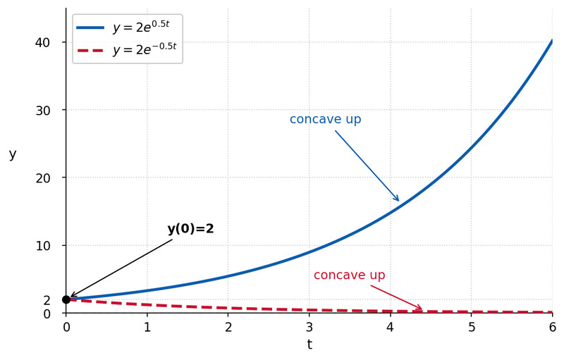
Exponential growth and decay with $y_0 = 2$

Notice both curves are concave up. Students sometimes think decay is concave down. It isn’t.

On FRQs, you may be asked what $\frac{dy}{dt} = ky$ means in words. A solid interpretation sounds like:

The rate at which the quantity changes is proportional to the amount present at time $t$.

Include units if given. If $y$ is in grams and $t$ in hours, then $k$ is per hour.

Finding $k$, predicting values, solving for time

Once you have
$y = y_0 e^{kt}$, everything becomes algebra.

Finding $k$

Suppose $y_0 = 500$ and $y(4) = 650$.

$$650 = 500e^{4k}$$

Divide:
$$1.3 = e^{4k}$$

Take ln:
$$\ln(1.3) = 4k \quad \Rightarrow \quad k = \frac{\ln(1.3)}{4}$$

Natural log is required because the model uses base $e$.

Solving for time

If you’re solving for $t$, same idea:

$$y = y_0 e^{kt}$$

1. Divide by $y_0$
2. Take ln
3. Solve for $t$

Logarithms are how you “bring down” the exponent.

Doubling time and half-life

These show up constantly.

Doubling time (growth, $k>0$)

Set $y = 2y_0$:

$$2 = e^{kt} \quad \Rightarrow \quad t = \frac{\ln 2}{k}$$

Half-life (decay, $k<0$)

Set $y = \frac{1}{2}y_0$:

$$\frac{1}{2} = e^{kt} \quad \Rightarrow \quad t = \frac{\ln(1/2)}{k}$$

Because $k$ is negative, time comes out positive.

The key idea: doubling time and half-life depend only on $k$, not on $y_0$.

Motion along a line

This model also applies to motion. If position $s(t)$ satisfies

$$\frac{ds}{dt} = ks$$

then velocity is proportional to position, and

$$s(t) = s_0 e^{kt}$$

Same math, different interpretation. On a test, you may need to say what the sign of $k$ implies about motion direction.