Topic 7.9 Notes – Logistic Models with Differential Equations

1. The Logistic Differential Equation

The logistic model comes from this statement:

The rate of change is jointly proportional to the size of the quantity and the difference between the quantity and the carrying capacity.

That translates to:

$$\frac{dy}{dt} = ky(M - y)$$

or equivalently,

$$\frac{dy}{dt} = ky\left(1 - \frac{y}{M}\right)$$

Where
- $y$ is the population (or quantity)
- $k > 0$ is a growth constant
- $M$ is the carrying capacity

What each factor means

• The $y$ factor makes growth proportional to current size. This is why small populations grow slowly and larger ones grow faster at first.
• The $(M - y)$ factor slows growth as the population approaches $M$.

When $y$ is small, $M - y \approx M$, so the model behaves almost like exponential growth.

When $y \to M$, the growth rate $\frac{dy}{dt} \to 0$.

That produces the classic S-shaped curve. Notice how the growth rate peaks in the middle and then decreases as the population levels off at the carrying capacity.

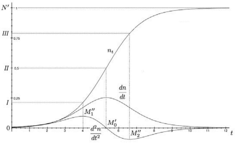
Logistic growth curve with first and second derivatives

2. Equilibrium Values and Carrying Capacity

Equilibrium solutions occur where the derivative equals zero.

$$ky(M - y) = 0$$

This gives:

• $y = 0$
• $y = M$

Both are equilibrium values, but only $M$ is the carrying capacity (the nonzero equilibrium).

Why $M$ is the carrying capacity

If you look at the sign of $\frac{dy}{dt}$:

• If $0 < y < M$, then $M - y > 0$, so $\frac{dy}{dt} > 0$ and the population increases.
• If $y > M$, then $M - y < 0$, so $\frac{dy}{dt} < 0$ and the population decreases.

Everything moves toward $M$. That means:

$$\lim_{t \to \infty} y(t) = M \quad \text{(if the initial population is positive)}$$

On FRQs, you are often given something like:

$$\frac{dy}{dt} = ay - by^2$$

Factor it:

$$\frac{dy}{dt} = y(a - by)$$

Set $a - by = 0$, and you get

$$M = \frac{a}{b}$$

Students often forget to factor first. If you cannot clearly see $M$, rewrite the equation.

3. When the Population Is Growing Fastest

Now think of the growth rate as a function of $y$:

$$\frac{dy}{dt} = ky(M - y)$$

As a function of $y$, this is a downward-opening quadratic with zeros at:

• $y = 0$
• $y = M$

The maximum of a quadratic occurs halfway between its zeros.

So the growth rate is largest at:

$$y = \frac{M}{2}$$

This is also the inflection point of the logistic curve.

• Below $M/2$ → concave up
• Above $M/2$ → concave down

On tests, once you find $M$, immediately think “fastest growth = $M/2$.” You do not need to solve the differential equation.

4. Interpreting Without Solving

You are rarely required to separate variables and solve the logistic equation on the AP exam. Most questions ask you to interpret from the model and initial condition.

Given $y(0) = y_0$:

• If $0 < y_0 < M$ → population increases toward $M$.
• If $y_0 > M$ → population decreases toward $M$.
• If $y_0 = M$ → constant solution.
• If $y_0 = 0$ → stays at 0.

You can justify all of this just by analyzing the sign of $ky(M - y)$. That reasoning earns points on FRQs.

5. Logistic vs Exponential Growth

Here is the clean comparison:

If a problem mentions limited resources, crowding, or maximum sustainable size, you are in logistic territory.